신용카드 사기 탐지(Kaggle)
신용카드 사기 탐지 (Credit Card Fraud Detection)
kaggle 에서 기존의 분석 경험 쌓기 + 프로그래밍 스킬 + 분석할 때 사용되는 영어 공부를 같이 진행합니다. 확실하게 진행되는 것이 우선순위인 속도로 진행됩니다.
- janiobachmann 님이 작성해주신 CODE를 필사합니다. 감사합니다.
Credit Fraud Detector
신용카드 사기 탐지
Note: There are still aspects of this kernel that will be subjected to changes. I’ve noticed a recent increase of interest towards this kernel so I will focus more on the steps I took and why I took them to make it clear why I took those steps.
메모: 이 커널에는 추가로 변경될 수 있는 측면이 여전히 있습니다. 최근 이 커널에 대한 관심이 증가하고 있다는 것을 알게 되었기 때문에 취한 조치와 그 이유를 명확히 하기 위해 취한 조치에 더 집중하겠습니다.
Before we Begin:
If you liked my work, please upvote this kernel since it will keep me motivated to perform more in-depth reserach towards this subject and will look for more efficient ways so that our models are able to detect more accurately both fraud and non-fraud transactions.
시작하기 전에
만약 이 작업이 좋다면, 이 커널을 추천해주세요. 이 커널은 제가 이 주제에 대해 더 심층적인 연구를 수행하도록 동기를 부여하고 모델이 사기 및 비사기 거래를 더 정확하게 탐지할 수 있도록 더 효율적인 방법을 찾을 것입니다.
Introduction
In this kernel we will use various predictive models to see how accurate they are in detecting whether a transaction is a normal payment or a fraud. As described in the dataset, the features are scaled and the names of the features are not shown due to privacy reasons. Nevertheless, we can still analyze some important aspects of the dataset. Let’s start!
소개
이 커널은 다양한 예측 모델을 사용하여 거래가 정상적인 지불인지 사기인지 탐지하는데 얼마나 정확한지 확인할 것입니다. 데이터 세트에 설명된 대로 요인의 크기가 조정되고 개인 정보 보호 문제로 인해 요인의 이름이 표시되지 않습니다. 그럼에도 불구하고, 우리는 여전히 데이터 세트의 몇 가지 중요한 측면을 분석할 수 있습니다. 시작해봅시다.
사기 거래에 대한 추가 설명으로 신용카드 회사가 고객이 구매하지 않은 항목에 대해서 사기 거래로 탐지하여 비용이 청구되지 않도록 하는 것입니다.
Our Goals:
- Understand the little distribution of the "little" data that was provided to us.
- Create a 50/50 sub-dataframe ratio of "Fraud" and "Non-Fraud" transactions. (NearMiss Algorithm)
- Determine the Classifiers we are going to use and decide which one has a higher accuracy.
- Create a Neural Network and compare the accuracy to our best classifier.
- Understand common mistaked made with imbalanced datasets.
목표
- 우리에게 제공된 작은 데이터의 작은 분포를 이해합니다.
- “Fraud” 와 “Non-Fraud” 거래의 50/50 하위 데이터 프레임 비율을 만듭니다. (NearMiss Algorithm)
- 사용할 분류자를 결정하고 정확도가 높은 분류자를 결정합니다.
- 신경망을 만들고 우리의 최고 분류기와 정확도를 비교합니다.
- 불균형 데이터셋으로 인한 일반적인 실수를 이해합니다.
Outline:
I. Understanding our data
a) Gather Sense of our data
II. Preprocessing
a) Scaling and Distributing
b) Splitting the Data
III. Random UnderSampling and Oversampling
a) Distributing and Correlating
b) Anomaly Detection
c) Dimensionality Reduction and Clustering (t-SNE)
d) Classifiers
e) A Deeper Look into Logistic Regression
f) Oversampling with SMOTE
IV. Testing
a) Testing with Logistic Regression
b) Neural Networks Testing (Undersampling vs Oversampling)
개요:
I. 데이터 이해하기
a) 데이터 의미 수집
II. 전처리
a) 스케일링 및 분산
b) 데이터 분할
III. 임의 언더샘플링과 오버샘플링Random UnderSampling and Oversampling
a) 분산과 상관관계
b) 이상 탐지
c) 차원 축소 및 클러스터링(t-SNE)
d) 분류기
e) 로지스틱 회귀 분석 더 자세히 보기
f) SMOTE로 오버샘플링
IV. 테스트
a) 로지스틱 회귀 분석을 사용한 검정
b) 신경망 테스트(언더샘플링 vs 오버샘플링)
Correcting Previous Mistakes from Imbalanced Datasets:
- Never test on the oversampled or undersampled dataset.
- If we want to implement cross validation, remember to oversample or undersample your training data during cross-validation, not before!
- Don't use accuracy score as a metric with imbalanced datasets (will be usually high and misleading), instead use f1-score, precision/recall score or confusion matrix
불균형 데이터 세트의 이전 실수 수정:
- 오버샘플링 또는 언더 샘플링 데이터 세트에서는 절대 테스트하지 하세요.
- 교차 검증을 구현하려면 교차 검증 중에 train 데이터를 과도하게 샘플링하거나 과소 샘플링하는 것을 잊지 마십시오. 이전에는 그렇지 않았습니다!
- 불균형 데이터 세트 matrix로 정확한(Accuracy) 점수를 사용하지 마십시오(일반적으로 높고 오해의 소지가 있음). 대신 f1 점수, 정밀도/호출 점수 또는 혼동 행렬(confusion matrix)을 사용하세요.
References:
- Hands on Machine Learning with Scikit-Learn & TensorFlow by Aurélien Géron (O'Reilly). CopyRight 2017 Aurélien Géron
- Machine Learning - Over-& Undersampling - Python/ Scikit/ Scikit-Imblearn by Coding-Maniac
- auprc, 5-fold c-v, and resampling methods by Jeremy Lane (Kaggle Notebook)
참고자료:
- Aurelien Géron(O’Reilly)의 Scikit-Learn & TensorFlow를 사용한 머신 러닝 실습. 저작권 2017 Aurelien Géron
- 기계 학습 - 오버&언더샘플링 - Python/Scikit/Scikit-Imblearn by Coding-Maniac
- by Jeremy Lane (Kaggle Notebook)
Gather Sense of Our Data:
The first thing we must do is gather a basic sense of our data. Remember, except for the transaction and amount we dont know what the other columns are (due to privacy reasons). The only thing we know, is that those columns that are unknown have been scaled already.
데이터를 이해하고 파악하기
우리가 가장 먼저 해야 할 일은 우리의 데이터에 대한 기본적인 정보를 수집하는 것입니다.
거래와 금액을 제외하고는 (개인 정보 보호상의 이유로) 다른 열이 무엇인지 알 수 없습니다.
알고 있는 열을 제외하고 모두 스케일링 되어 있다는 것을 알 수 있습니다.
Summary:
- The transaction amount is relatively small. The mean of all the amounts made is approximately USD 88.
- There are no "Null" values, so we don't have to work on ways to replace values.
- Most of the transactions were Non-Fraud (99.83%) of the time, while Fraud transactions occurs (017%) of the time in the dataframe.
요약:
- 이 데이터 세트에서 모든 거래 금액의 평균은 대략 88달러로 비교적 적은 금액으로 이루어져 있습니다.
- “Null”값이 없으므로 값을 대체할 방법을 강구할 필요가 없습니다.
- 이 데이터프레임에서는 대부분의 거래는 ‘Non-Fraud’(99.83%) 이며, ‘Fraud’(0.17%) 로 나타납니다.
Feature Technicalities:
- PCA Transformation: The description of the data says that all the features went through a PCA transformation (Dimensionality Reduction technique) (Except for time and amount).
- Scaling: Keep in mind that in order to implement a PCA transformation features need to be previously scaled. (In this case, all the V features have been scaled or at least that is what we are assuming the people that develop the dataset did.)
독립변수 기술:
- PCA 변환
- 데이터 설명에 따르면 모든 독립변수가 PCA 변환(차원 축소 기법)을 거쳤다고 합니다.(Time과 Amount는 제외)
- 스케일링
- PCA 변환 기능을 구현하려면 사전에 스케일링 해야합니다. (이 경우에는 모든 V 독립변수가 스케일링 되었거나 적어도 데이터셋을 개발한 사람들이 그렇게 가정한다는 것입니다.)
# Imported Libraries
import numpy as np
import pandas as pd
import tensorflow as tf
import matplotlib.pyplot as plt
import seaborn as sns
from sklearn.manifold import TSNE
from sklearn.decomposition import PCA, TruncatedSVD
import matplotlib.patches as mpatches # 도형으로 시각화 하는 것
import time

# Classifier Libraries
from sklearn.linear_model import LogisticRegression # 로지스틱 회귀
from sklearn.svm import SVC # 서포트벡터머신
from sklearn.neighbors import KNeighborsClassifier # K means 알고리즘
from sklearn.tree import DecisionTreeClassifier # 의사결정트리
from sklearn.ensemble import RandomForestClassifier # 랜덤포레스트 분류기
import collections # 컨테이너 데이터형

# Other Libraries
from sklearn.model_selection import train_test_split # 학습, 테스트 데이터 분리
from sklearn.pipeline import make_pipeline # sklearn 파이프라인
from imblearn.pipeline import make_pipeline as imbalanced_make_pipeline # 불균형 데이터 세트 다루기
from imblearn.over_sampling import SMOTE # 오버샘플링
from imblearn.under_sampling import NearMiss # 언더샘플링
from imblearn.metrics import classification_report_imbalanced #
from sklearn.metrics import precision_score, recall_score, f1_score, roc_auc_score, accuracy_score, classification_report
from collections import Counter
from sklearn.model_selection import KFold, StratifiedKFold
import warnings
warnings.filterwarnings("ignore")

df = pd.read_csv("../../archive/data/신용카드사기탐지/creditcard.csv")
display(df.describe())
출력 보기(클릭)
| Time | V1 | V2 | V3 | V4 | V5 | V6 | V7 | V8 | V9 | ... | V21 | V22 | V23 | V24 | V25 | V26 | V27 | V28 | Amount | Class | |
|---|---|---|---|---|---|---|---|---|---|---|---|---|---|---|---|---|---|---|---|---|---|
| count | 284807.000000 | 2.848070e+05 | 2.848070e+05 | 2.848070e+05 | 2.848070e+05 | 2.848070e+05 | 2.848070e+05 | 2.848070e+05 | 2.848070e+05 | 2.848070e+05 | ... | 2.848070e+05 | 2.848070e+05 | 2.848070e+05 | 2.848070e+05 | 2.848070e+05 | 2.848070e+05 | 2.848070e+05 | 2.848070e+05 | 284807.000000 | 284807.000000 |
| mean | 94813.859575 | 3.918649e-15 | 5.682686e-16 | -8.761736e-15 | 2.811118e-15 | -1.552103e-15 | 2.040130e-15 | -1.698953e-15 | -1.893285e-16 | -3.147640e-15 | ... | 1.473120e-16 | 8.042109e-16 | 5.282512e-16 | 4.456271e-15 | 1.426896e-15 | 1.701640e-15 | -3.662252e-16 | -1.217809e-16 | 88.349619 | 0.001727 |
| std | 47488.145955 | 1.958696e+00 | 1.651309e+00 | 1.516255e+00 | 1.415869e+00 | 1.380247e+00 | 1.332271e+00 | 1.237094e+00 | 1.194353e+00 | 1.098632e+00 | ... | 7.345240e-01 | 7.257016e-01 | 6.244603e-01 | 6.056471e-01 | 5.212781e-01 | 4.822270e-01 | 4.036325e-01 | 3.300833e-01 | 250.120109 | 0.041527 |
| min | 0.000000 | -5.640751e+01 | -7.271573e+01 | -4.832559e+01 | -5.683171e+00 | -1.137433e+02 | -2.616051e+01 | -4.355724e+01 | -7.321672e+01 | -1.343407e+01 | ... | -3.483038e+01 | -1.093314e+01 | -4.480774e+01 | -2.836627e+00 | -1.029540e+01 | -2.604551e+00 | -2.256568e+01 | -1.543008e+01 | 0.000000 | 0.000000 |
| 25% | 54201.500000 | -9.203734e-01 | -5.985499e-01 | -8.903648e-01 | -8.486401e-01 | -6.915971e-01 | -7.682956e-01 | -5.540759e-01 | -2.086297e-01 | -6.430976e-01 | ... | -2.283949e-01 | -5.423504e-01 | -1.618463e-01 | -3.545861e-01 | -3.171451e-01 | -3.269839e-01 | -7.083953e-02 | -5.295979e-02 | 5.600000 | 0.000000 |
| 50% | 84692.000000 | 1.810880e-02 | 6.548556e-02 | 1.798463e-01 | -1.984653e-02 | -5.433583e-02 | -2.741871e-01 | 4.010308e-02 | 2.235804e-02 | -5.142873e-02 | ... | -2.945017e-02 | 6.781943e-03 | -1.119293e-02 | 4.097606e-02 | 1.659350e-02 | -5.213911e-02 | 1.342146e-03 | 1.124383e-02 | 22.000000 | 0.000000 |
| 75% | 139320.500000 | 1.315642e+00 | 8.037239e-01 | 1.027196e+00 | 7.433413e-01 | 6.119264e-01 | 3.985649e-01 | 5.704361e-01 | 3.273459e-01 | 5.971390e-01 | ... | 1.863772e-01 | 5.285536e-01 | 1.476421e-01 | 4.395266e-01 | 3.507156e-01 | 2.409522e-01 | 9.104512e-02 | 7.827995e-02 | 77.165000 | 0.000000 |
| max | 172792.000000 | 2.454930e+00 | 2.205773e+01 | 9.382558e+00 | 1.687534e+01 | 3.480167e+01 | 7.330163e+01 | 1.205895e+02 | 2.000721e+01 | 1.559499e+01 | ... | 2.720284e+01 | 1.050309e+01 | 2.252841e+01 | 4.584549e+00 | 7.519589e+00 | 3.517346e+00 | 3.161220e+01 | 3.384781e+01 | 25691.160000 | 1.000000 |
8 rows × 31 columns
# Null 값 확인하기
print(df.isnull().sum().max())
0
# 독립변수 확인하기
df.columns
Index(['Time', 'V1', 'V2', 'V3', 'V4', 'V5', 'V6', 'V7', 'V8', 'V9', 'V10',
       'V11', 'V12', 'V13', 'V14', 'V15', 'V16', 'V17', 'V18', 'V19', 'V20',
       'V21', 'V22', 'V23', 'V24', 'V25', 'V26', 'V27', 'V28', 'Amount',
       'Class'],
      dtype='object')
# 클래스가 심하게 기울어져 있어 이 문제를 나중에 해결해야합니다.
print(f"No Fraud {round(df['Class'].value_counts()[0]/len(df) * 100,2)}% of the dataset")
print(f"Frauds {round(df['Class'].value_counts()[1]/len(df) * 100,2)}% of the dataset")
No Fraud 99.83% of the dataset
Frauds 0.17% of the dataset
Note: Notice how imbalanced is our original dataset! Most of the transactions are non-fraud. If we use this dataframe as the base for our predictive models and analysis we might get a lot of errors and our algorithms will probably overfit since it will “assume” that most transactions are not fraud. But we don’t want our model to assume, we want our model to detect patterns that give signs of fraud!
메모: 원본 데이터 세트가 얼마나 불균형적인지 주목하십시오! 대부분의 거래는 사기가 아닙니다. 이 데이터 프레임을 예측 모델 및 분석의 기반으로 사용하면 많은 오류가 발생할 수 있으며 대부분의 거래가 사기가 아니라고 “assume”하기 때문에 알고리즘이 과도하게 적합할 수 있습니다. 하지만 우리는 모델이 사기를 탐지하기 위해 특정한 패턴을 학습하도록 하는 것이 목적입니다.
# Class 열의 데이터 분포를 막대그래프로 시각하화여 차이를 확인합니다.
colors = ['#0101DF','#DF0101']

sns.countplot(data = df, x = "Class", palette = colors)
plt.title('Class Distributions \n (0: No Fraud || 1: Fraud)', fontsize=14)
plt.show()


Distributions: By seeing the distributions we can have an idea how skewed are these features, we can also see further distributions of the other features. There are techniques that can help the distributions be less skewed which will be implemented in this notebook in the future.
분포: 분포를 보면 이러한 형상이 얼마나 치우쳐 있는지 알 수 있고, 다른 형태의 추가 분포도 볼 수 있습니다. 분포의 왜곡을 줄이는 데 도움이 되는 기술이 있으며, 향후 이 노트북에 구현될 예정입니다.
# Amount, Time 열을 histogram 그래프로 각 열의 데이터 분포를 살펴봅니다. 얼마나 모여있거나 치우쳐졌는지 확인합니다.
fig, ax = plt.subplots(1, 2, figsize=(18,4))

amount_val = df['Amount'].values
time_val = df['Time'].values

sns.distplot(amount_val, ax=ax[0], color='r')
ax[0].set_title("Distribution of Transaction Amount", fontsize=14)
ax[0].set_xlim([min(amount_val), max(amount_val)])

sns.distplot(time_val, ax=ax[1], color='b')
ax[1].set_title('Distribution of Transaction Time', fontsize=14)
ax[1].set_xlim([min(time_val), max(time_val)])

plt.show()


Scaling and Distributing
In this phase of our kernel, we will first scale the columns comprise of Time and Amount . Time and amount should be scaled as the other columns. On the other hand, we need to also create a sub sample of the dataframe in order to have an equal amount of Fraud and Non-Fraud cases, helping our algorithms better understand patterns that determines whether a transaction is a fraud or not.
스케일링과 분산
컨널의 이 단계에서는 먼저 Time과 Amount로 구성된 열을 확장합니다. 시간과 양은 다른 열과 마찬가지로 스케일링 되어야 합니다. 다른 한편으로, 우리는 동일한 양의 Fraud 및 Non-Fraud 사례를 보유하기 위해 DataFrame의 하위 샘플을 생성해야 하며, 이는 우리의 알고리즘이 거래가 Fraud인지 여부를 결정하는 패턴을 더 잘 이해할 수 있도록 도와줍니다.
What is a sub-Sample?
In this scenario, our subsample will be a dataframe with a 50/50 ratio of fraud and non-fraud transactions. Meaning our sub-sample will have the same amount of fraud and non fraud transactions.
하위 샘플은 무엇인가?
이 시나리오에서 우리의 서브샘플은 Fraud 와 Non-Fraud의 비율이 50/50 인 데이터 프레임이 될 것입니다. 즉, 하위 샘플은 동일한 양의 Fraud와 Non-Fraud 를 하게 됩니다.
Why do we create a sub-Sample?
In the beginning of this notebook we saw that the original dataframe was heavily imbalanced! Using the original dataframe will cause the following issues:
- Overfitting: Our classification models will assume that in most cases there are no frauds! What we want for our model is to be certain when a fraud occurs.
- Wrong Correlations: Although we don't know what the "V" features stand for, it will be useful to understand how each of this features influence the result (Fraud or No Fraud) by having an imbalance dataframe we are not able to see the true correlations between the class and features.
하위 샘플은 왜 만드는 것인가?
시작 부분에서 원본 데이터 프레임의 불균형이 심각하다는 것을 알 수 있었습니다. 원래 데이터 프레임을 사용하면 다음과 같은 문제가 발생합니다.
- 과적합
- 우리의 분류 모델은 대부분의 경우 사기가 없다고 가정할 것입니다! 우리가 모델에 대해 원하는 것은 사기가 발생했을 때 확실하게 하는 것입니다.
- 잘못된 상관 관계
- “V” 독립변수가 무엇을 의미하는지는 알 수 없지만, 종속변수와 독립변수 간의 실제 상관 관계를 확인할 수 없는 불균형 데이터 프레임을 사용하여 이러한 각 기능이 결과(사기 또는 사이 없음)에 어떤 영향을 미치는지 이해하는 것이 유용할 것입니다.
Summary:
- Scaled amount and scaled time are the columns with scaled values.
- There are 492 cases of fraud in our dataset so we can randomly get 492 cases of non-fraud to create our new sub dataframe.
- We concat the 492 cases of fraud and non fraud, creating a new sub-sample.
요약:
- 스케일화된 “Amount” 와 스케일화된 “Time” 은 스케일화된 값을 갖는 열입니다.
- 데이터 세트에는 492 건의 Fraud 사례가 있으므로 492 건의 Non-Fraud 사례를 무작위로 받아 새로운 하위 데이터 프레임을 만들 수 있습니다.
- 우리는 492건의 Fraud 및 Non-Fraud 사례를 결합하여 새로운 하위 샘플을 생성합니다.
# 데이터의 대부분이 이미 확장되었기 때문에 남은 열을 확장해야 합니다.(Amount and Time)

from sklearn.preprocessing import StandardScaler, RobustScaler

# RobustScaler는 이상값에 덜 취약합니다. 따라서 이번 장에서는 RobustScaler를 사용합니다.

std_scaler = StandardScaler()
rob_scaler = RobustScaler()

df['scaled_amount'] = rob_scaler.fit_transform(df['Amount'].values.reshape(-1,1))
df['scaled_time'] = rob_scaler.fit_transform(df['Time'].values.reshape(-1,1))

df.drop(['Amount', 'Time'], axis=1, inplace=True)
# 스케일화 된 열들을 교체해줍니다.
scaled_amount = df['scaled_amount']
scaled_time = df['scaled_time']

df.drop(['scaled_amount', 'scaled_time'], axis=1, inplace=True)
df.insert(0, 'scaled_amount', scaled_amount)
df.insert(1, 'scaled_time', scaled_time)

# Amount and Time are Scaled!

display(df.head())
출력 보기(클릭)
| scaled_amount | scaled_time | V1 | V2 | V3 | V4 | V5 | V6 | V7 | V8 | ... | V20 | V21 | V22 | V23 | V24 | V25 | V26 | V27 | V28 | Class | |
|---|---|---|---|---|---|---|---|---|---|---|---|---|---|---|---|---|---|---|---|---|---|
| 0 | 1.783274 | -0.994983 | -1.359807 | -0.072781 | 2.536347 | 1.378155 | -0.338321 | 0.462388 | 0.239599 | 0.098698 | ... | 0.251412 | -0.018307 | 0.277838 | -0.110474 | 0.066928 | 0.128539 | -0.189115 | 0.133558 | -0.021053 | 0 |
| 1 | -0.269825 | -0.994983 | 1.191857 | 0.266151 | 0.166480 | 0.448154 | 0.060018 | -0.082361 | -0.078803 | 0.085102 | ... | -0.069083 | -0.225775 | -0.638672 | 0.101288 | -0.339846 | 0.167170 | 0.125895 | -0.008983 | 0.014724 | 0 |
| 2 | 4.983721 | -0.994972 | -1.358354 | -1.340163 | 1.773209 | 0.379780 | -0.503198 | 1.800499 | 0.791461 | 0.247676 | ... | 0.524980 | 0.247998 | 0.771679 | 0.909412 | -0.689281 | -0.327642 | -0.139097 | -0.055353 | -0.059752 | 0 |
| 3 | 1.418291 | -0.994972 | -0.966272 | -0.185226 | 1.792993 | -0.863291 | -0.010309 | 1.247203 | 0.237609 | 0.377436 | ... | -0.208038 | -0.108300 | 0.005274 | -0.190321 | -1.175575 | 0.647376 | -0.221929 | 0.062723 | 0.061458 | 0 |
| 4 | 0.670579 | -0.994960 | -1.158233 | 0.877737 | 1.548718 | 0.403034 | -0.407193 | 0.095921 | 0.592941 | -0.270533 | ... | 0.408542 | -0.009431 | 0.798278 | -0.137458 | 0.141267 | -0.206010 | 0.502292 | 0.219422 | 0.215153 | 0 |
5 rows × 31 columns
Splitting the Data (Original DataFrame)
Before proceeding with the Random UnderSampling technique we have to separate the orginal dataframe. Why? for testing purposes, remember although we are splitting the data when implementing Random UnderSampling or OverSampling techniques, we want to test our models on the original testing set not on the testing set created by either of these techniques. The main goal is to fit the model either with the dataframes that were undersample and oversample (in order for our models to detect the patterns), and test it on the original testing set.
데이터 분리 ( 원본 데이터 프레임 )
랜덤 언더샘플링 기법을 진행하기 전에 원본 데이터 프레임을 분리해야 합니다. 왜 그럴까요?
테스트 목적으로 랜덤 언더샘플링 또는 오버샘플링 기법을 구현할 때 데이터를 분할하지만 이러한 기법으로 생성된 테스트 세트가 아닌 원래 테스트 세트에서 모델을 테스트하고자 합니다.
주요 목표는 모델을 언더샘플 및 오버샘플 데이터 프레임(모델이 패턴을 감지할 수 있도록)에 맞추고 원래 테스트 세트에서 테스트하는 것입니다.
from sklearn.model_selection import train_test_split
from sklearn.model_selection import StratifiedShuffleSplit # 비율을 맞추어 데이터를 분리할 수 있는 라이브러리입니다.

# Class에 대한 Fraud 대 Non-Fraud의 비율을 구합니다.
print(f"No Frauds {round(df['Class'].value_counts()[0]/len(df) * 100,2)}% of the dataset")
print(f"Frauds {round(df['Class'].value_counts()[1]/len(df) * 100, 2)}% of the dataset")

# 독립변수와 종속변수를 나눕니다.
X = df.drop('Class', axis = 1)
y = df['Class']

# 데이터세트를 5개의 Fold로 나누어줍니다.
sss = StratifiedKFold(n_splits=5, random_state=None, shuffle=False)

# v
for train_index, test_index in sss.split(X,y):
    print("Train:", train_index, "Test:", test_index)
    original_Xtrain, original_Xtest = X.iloc[train_index], X.iloc[test_index]
    original_ytrain, original_ytest = y.iloc[train_index], y.iloc[test_index]

# 우리는 이미 하위 샘플 데이터를 위한 X_train과 y_train을 가지고 있기 때문에 이 변수들을 구별하고 덮어쓰지 않기 위해 원본을 사용하고 있습니다.
# original_Xtrain, original_Xtest, original_ytrain, original_ytest

# 레이블 분포 확인

# 배열로 바꾼다.
original_Xtrain = original_Xtrain.values
original_Xtest = original_Xtest.values
original_ytrain = original_ytrain.values
original_ytest = original_ytest.values

# 학습, 테스트 라벨 분포가 유사한지 확인
train_unique_label, train_counts_label = np.unique(original_ytrain, return_counts=True)
test_unique_label, test_counts_label = np.unique(original_ytest, return_counts=True)
print('-'*100)

print('Label Distributions: \n')
print(train_counts_label/len(original_ytrain))
print(test_counts_label/len(original_ytest))
No Frauds 99.83% of the dataset
Frauds 0.17% of the dataset
Train: [ 30473  30496  31002 ... 284804 284805 284806] Test: [    0     1     2 ... 57017 57018 57019]
Train: [     0      1      2 ... 284804 284805 284806] Test: [ 30473  30496  31002 ... 113964 113965 113966]
Train: [     0      1      2 ... 284804 284805 284806] Test: [ 81609  82400  83053 ... 170946 170947 170948]
Train: [     0      1      2 ... 284804 284805 284806] Test: [150654 150660 150661 ... 227866 227867 227868]
Train: [     0      1      2 ... 227866 227867 227868] Test: [212516 212644 213092 ... 284804 284805 284806]
----------------------------------------------------------------------------------------------------
Label Distributions:

[0.99827076 0.00172924]
[0.99827952 0.00172048]
Random Under-Sampling:
In this phase of the project we will implement “Random Under Sampling” which basically consists of removing data in order to have a more balanced dataset and thus avoiding our models to overfitting.
프로젝트의 이 단계에서 우리는 임의 하위 샘플링을 구현할 것입니다. 이는 기본적으로 데이터를 제거하여 보다 균형 잡힌 데이터 세트를 보유하고 모델이 과적합되는 것을 방지하는 것으로 구성됩니다.
Steps:
- The first thing we have to do is determine how imbalanced is our class (use "value_counts()" on the class column to determine the amount for each label)
- Once we determine how many instances are considered fraud transactions (Fraud = "1") , we should bring the non-fraud transactions to the same amount as fraud transactions (assuming we want a 50/50 ratio), this will be equivalent to 492 cases of fraud and 492 cases of non-fraud transactions.
- After implementing this technique, we have a sub-sample of our dataframe with a 50/50 ratio with regards to our classes. Then the next step we will implement is to shuffle the data to see if our models can maintain a certain accuracy everytime we run this script.
단계:
- 첫번째로 클래스가 얼마나 불균형인지를 결정하는 것입니다. ( 클래스 열에서 “value_counts()” 를 사용하여 각 레이블의 양을 결정 )
- “Fraud”로 간주되는 사례가 얼마나 되는지를 파악하면 ( Fraud = ‘1’ ), “Non-Fraud”를 “Fraud”와 동일한 양(50/50 비율을 원한다고 가정하면), 이는 “Fraud” 492건, “Non-Fraud” 492건에 해당합니다.
- 이 기술을 구현한 후, 클래스와 관련하여 50/50 비율의 데이터 프레임의 하위 샘픙을 갖게 됩니다. 그런 다음 구현할 다음 단계는 이 스크립트를 실행할 때마다 모델이 일정한 정확도를 유지할 수 있는지 확인하기 위해 데이터를 섞는 것입니다.
Note: The main issue with “Random Under-Sampling” is that we run the risk that our classification models will not perform as accurate as we would like to since there is a great deal of information loss (bringing 492 non-fraud transaction from 284,315 non-fraud transaction)
메모:
- 임의 언더샘플링의 주요 문제는 엄청난 양의 정보 손실(284,315개의 “Non-Fraud” 거래에서 492개의 거래 발생)이 있기 때문에 분류 모델이 원하는 만큼 정확하게 수행되지 않을 위험이 있다는 것입니다.
# 클래스가 심하게 치우쳐 있으므로 클래스의 정규 분포를 얻으려면 클래스를 동등하게 만들어야 합니다.

# 하위 샘플을 만들기 전에 데이터를 섞습니다.
df = df.sample(frac=1)

# 492 건의 Fraud와 Non-Fraud의 클래스 정의
fraud_df = df.loc[df['Class'] == 1]
non_fraud_df = df.loc[df['Class'] == 0][:492] # Non-fraud의 데이터의 개수는 많습니다. 그 중 fraud의 데이터의 개수와 같은 492 개의 데이터만 인덱싱해줍니다.

normal_distributed_df = pd.concat([fraud_df,non_fraud_df]) # 위 두개의 데이터 프레임을 결합하여 fraud와 non-fraud의 데이터 비율이 비슷하게 분포한 데이터 프레임을 만들어 줍니다.

# 데이터 행의 순서를 섞는다.
new_df = normal_distributed_df.sample(frac=1,random_state=42)

new_df.head()
출력 보기(클릭)
| scaled_amount | scaled_time | V1 | V2 | V3 | V4 | V5 | V6 | V7 | V8 | ... | V20 | V21 | V22 | V23 | V24 | V25 | V26 | V27 | V28 | Class | |
|---|---|---|---|---|---|---|---|---|---|---|---|---|---|---|---|---|---|---|---|---|---|
| 68789 | 0.158597 | -0.370669 | -0.719391 | -0.048663 | 1.490211 | -0.370573 | 0.534053 | 0.035476 | 0.131233 | 0.361854 | ... | -0.038740 | -0.145766 | -0.554125 | 0.071964 | -0.316707 | -0.002313 | 0.171520 | -0.078408 | -0.043258 | 0 |
| 183106 | -0.307413 | 0.481279 | 0.224414 | 2.994499 | -3.432458 | 3.986519 | 3.760233 | 0.165640 | 1.099378 | -0.654557 | ... | -0.200846 | 0.491337 | -0.984223 | -0.421979 | -1.048058 | 0.726412 | 0.268625 | 0.283689 | 0.419102 | 1 |
| 199649 | 0.725215 | 0.568345 | 1.840359 | -0.328201 | -1.443581 | 0.605344 | -0.024695 | -0.361448 | -0.256120 | 0.110281 | ... | -0.119201 | -0.034598 | -0.228939 | 0.201407 | 0.575203 | -0.321012 | 0.168316 | -0.052961 | -0.020989 | 0 |
| 263877 | -0.302103 | 0.898295 | -3.387601 | 3.977881 | -6.978585 | 1.657766 | -1.100500 | -3.599487 | -3.686651 | 1.942252 | ... | -0.004301 | 1.043587 | 0.262189 | -0.479224 | -0.326638 | -0.156939 | 0.113807 | 0.354124 | 0.287592 | 1 |
| 248296 | -0.307413 | 0.812780 | -0.613696 | 3.698772 | -5.534941 | 5.620486 | 1.649263 | -2.335145 | -0.907188 | 0.706362 | ... | 0.354773 | 0.319261 | -0.471379 | -0.075890 | -0.667909 | -0.642848 | 0.070600 | 0.488410 | 0.292345 | 1 |
5 rows × 31 columns
Equally Distributing and Correlating:
Now that we have our dataframe correctly balanced, we can go further with our analysis and data preprocessing.
균등 분산과 상관관계
이제 데이터프레임의 균형이 올바르게 조정되었으므로 분석과 데이터 전처리를 더 진행할 수 있습니다.
print("Distribution of the Classes in the subsample dataset")
print(new_df['Class'].value_counts()/len(new_df))
Distribution of the Classes in the subsample dataset
0    0.5
1    0.5
Name: Class, dtype: float64
sns.countplot(data=new_df, x="Class", palette=colors)
plt.title("Equally Distributed Classed", fontsize=14)
plt.show()


Correlation Matrices
Correlation matrices are the essence of understanding our data. We want to know if there are features that influence heavily in whether a specific transaction is a fraud. However, it is important that we use the correct dataframe (subsample) in order for us to see which features have a high positive or negative correlation with regards to fraud transactions.
상관 행렬
- 상관 행렬은 데이터를 이행하는 데 필수적인 요소입니다. 특정 거래가 사기인지 여부에 큰 영향을 미치는 독립 변수가 있는지 알고 싶습니다. 그러나 “Fraud” 거래와 관련하여 어떤 독립변수가 높은 양 또는 음의 상관관계를 가지는지 확인하려면 올바른 데이터 프레임(하위 샘플)을 사용하는 것이 중요합니다.
Summary and Explanation:
- Negative Correlations: V17, V14, V12 and V10 are negatively correlated. Notice how the lower these values are, the more likely the end result will be a fraud transaction.
- Positive Correlations: V2, V4, V11, and V19 are positively correlated. Notice how the higher these values are, the more likely the end result will be a fraud transaction.
- BoxPlots: We will use boxplots to have a better understanding of the distribution of these features in fradulent and non fradulent transactions.
요약 및 설명:
- 음의 상관관계 : V17, V14, V12, V10은 음의 상관관계가 있습니다. 이러한 값이 낮을수록 최종 결과는 “Fraud” 거래가 될 가능성이 높습니다.
- 양의 상관관계 : V2, V4, V11, V19는 양의 상관관계가 있습니다. 이러한 값이 높을수록 최종 결과가 “Fraud” 거래로 이러질 가능성이 높아집니다.
- 상자 그림(Boxplot) : 상자 그림을 사용하여 “Fraud” 및 “Non-Fraud” 거래에서 이러한 독립변수의 분포를 더 잘 이해할 것입니다.
Note: We have to make sure we use the subsample in our correlation matrix or else our correlation matrix will be affected by the high imbalance between our classes. This occurs due to the high class imbalance in the original dataframe.
메모:
- 상관 행렬에는 하위 샘플을 사용해야 합니다. 그렇지 않으면 상관 행렬은 클래스 간의 높은 불균형의 영향을 받을 것입니다. 이 문제는 원래 데이터 프레임의 높은 클래스 불균형 때문에 발생합니다.
# 상관관계에서는 하위 샘플을 이용해야 합니다.
f, (ax1, ax2) = plt.subplots(2, 1, figsize=(24,20))

# 전체 데이터프레임
corr = df.corr()
sns.heatmap(corr, cmap='coolwarm_r', annot_kws={'size':20}, ax=ax1)
ax1.set_title("Imbalanced Correlation Matrix \n (don't use for reference)", fontsize = 14)

sub_sample_corr = new_df.corr()
sns.heatmap(sub_sample_corr, cmap='coolwarm_r', annot_kws={"size":20}, ax=ax2)
ax2.set_title("SubSample Correlation Matrix \n (use for reference)", fontsize = 14)
plt.show()


f, axes = plt.subplots(ncols=4, figsize=(20,4))

# 클래스와의 부정적인 상관 관계 ( 독립 변수 값이 낮을수록 "Fraud" 거래일 가능성이 높음 )

sns.boxplot(x='Class', y = 'V17', data=new_df, palette=colors, ax=axes[0])
axes[0].set_title('V17 vs Class Negative Correlation')

sns.boxplot(x='Class', y = 'V14', data = new_df, palette= colors, ax=axes[1])
axes[1].set_title('V14 vs Class Negative Correlation')

sns.boxplot(x='Class', y = 'V12', data = new_df, palette=colors, ax=axes[2])
axes[2].set_title('V12 vs Class Negative Correlation')

sns.boxplot(x='Class', y = 'V10', data = new_df, palette= colors, ax = axes[3])
axes[3].set_title('V10 vs Class Negative Correlation')

plt.show()


f, axes = plt.subplots(ncols=4, figsize=(20,4))

# 양의 상관관계 ( 독립변수 값이 높을수록 "Fraud" 거래일 확률이 증가합니다. )
sns.boxplot(x='Class', y='V11', data= new_df, palette=colors, ax=axes[0])
axes[0].set_title('V11 vs Class Positive Correlation')

sns.boxplot(x='Class', y= 'V4', data=new_df, palette=colors, ax=axes[1])
axes[1].set_title('V4 vs Class Positive Correlation')

sns.boxplot(x='Class', y='V2', data=new_df, palette=colors, ax=axes[2])
axes[2].set_title('V2 vs Class Positive Correlation')

sns.boxplot(x='Class', y='V19', data=new_df, palette=colors, ax=axes[3])
axes[3].set_title('V19 vs Class Positive Correlation')

plt.show()


Anomaly Detection:
Our main aim in this section is to remove “extreme outliers” from features that have a high correlation with our classes. This will have a positive impact on the accuracy of our models.
이상치 탐지:
이 센션의 주요 목표는 클래스와 상관관계가 높은 독립변수에서 ‘극단적인 이상값’을 제거하는 것입니다. 이렇게 하면 모델의 정확도에 긍정적인 영향을 미칩니다.
Interquartile Range Method:
- Interquartile Range (IQR): We calculate this by the difference between the 75th percentile and 25th percentile. Our aim is to create a threshold beyond the 75th and 25th percentile that in case some instance pass this threshold the instance will be deleted.
- Boxplots: Besides easily seeing the 25th and 75th percentiles (both end of the squares) it is also easy to see extreme outliers (points beyond the lower and higher extreme).
사분위간 범위 방법:
- 사분위간 범위(IQR):
- 75번째 백분위수와 25번째 백분위수의 차이로 계산합니다.
- 목표는 75번째 백분위수와 25번째 백분위수를 넘어서는 임계값을 생성하여 일부 인스턴스가 이 임계값을 통과할 경우 인스턴스가 삭제되도록 하는 것입니다.
- 상자 그림:
- 25번째 및 75번째 백분위수(사각형의 양쪽 끝)를 쉽게 볼 수 있을 뿐만 아니라 극단값 이상값(극단의 하한과 상한을 넘는 지점)도 쉽게 볼 수 있습니다.
Outlier Removal Tradeoff:
We have to be careful as to how far do we want the threshold for removing outliers. We determine the threshold by multiplying a number (ex: 1.5) by the (Interquartile Range). The higher this threshold is, the less outliers will detect (multiplying by a higher number ex: 3), and the lower this threshold is the more outliers it will detect.
이상값 제거 균형 맞추기:
이상값을 제거하기 위한 임계값을 어디까지 설정할지 신중하게 결정해야 합니다.
임계값은 숫자(예:1.5)에 사분위수 범위(IQR)를 곱하여 결정합니다. 이 임계값이 높을수록 더 적은 수의 이상값을 감지하고 낮을수록 더 많은 이상값을 감지합니다.
The Tradeoff:
The lower the threshold the more outliers it will remove however, we want to focus more on “extreme outliers” rather than just outliers. Why? because we might run the risk of information loss which will cause our models to have a lower accuracy. You can play with this threshold and see how it affects the accuracy of our classification models.
The Tradeoff:
임계값이 낮을수록 더 많은 이상값을 제거할 수 있지만, 단순한 이상값보다는 ‘극단적인 이상값’에 더 초점을 맞추고자 합니다.
그 이유는 정보 손실의 위험이 있어 모델의 정확도가 낮아질 수 있기 때문입니다. 이 임계값을 조절하면서 분류 모델의 정확도에 어떤 영향을 미치는지 확인할 수 있습니다.
Summary:
- Visualize Distributions: We first start by visualizing the distribution of the feature we are going to use to eliminate some of the outliers. V14 is the only feature that has a Gaussian distribution compared to features V12 and V10.
- Determining the threshold: After we decide which number we will use to multiply with the iqr (the lower more outliers removed), we will proceed in determining the upper and lower thresholds by substrating q25 - threshold (lower extreme threshold) and adding q75 + threshold (upper extreme threshold).
- Conditional Dropping: Lastly, we create a conditional dropping stating that if the "threshold" is exceeded in both extremes, the instances will be removed.
- Boxplot Representation: Visualize through the boxplot that the number of "extreme outliers" have been reduced to a considerable amount.
요약:
- 분포 시각화(Visualize Distributions):
- 일부 이상값을 제거하는 데 사용할 특징의 분포를 시각화하는 것으로 시작합니다.
- V14는 독립변수 V12 및 V10에 비해 가우스 분포를 갖는 유일한 특징입니다.
- 임계값 결정(Determining the threshold):
- IQR(더 많은 이상값을 제거할수록 낮은 IQR)을 곱하는 데 사용할 숫자를 결정한 후, q25 - 임계값(하한 임계값)과 q75 + 임계값(상한 임계값)을 더하여 상한 및 하한 임계값을 결정할 것입니다.
- 조건부 삭제(Conditional Dropping):
- 마지막으로, 양쪽 극단 모두에서 ‘임계값’을 초과하면 인스턴스를 제거한다는 조건부 삭제가 생성됩니다.
- 상자 그림 표현(Boxplot Representation):
- 상자 그림 표현을 통해 ‘극단값 이상값’의 수가 상당량 감소했음을 시각화합니다.
Note: After implementing outlier reduction our accuracy has been improved by over 3%! Some outliers can distort the accuracy of our models but remember, we have to avoid an extreme amount of information loss or else our model runs the risk of underfitting.
메모: 이상값 감소를 구현한 후 정확도가 3% 이상 향상되었습니다. 일부 이상값은 모델의 정확도를 왜곡할 수 있지만, 극단적인 정보 손실을 피하지 않으면 모델이 과소 적할될 위험이 있다는 점을 기억하세요.
Reference: More information on Interquartile Range Method: How to Use Statistics to Identify Outliers in Data by Jason Brownless (Machine Learning Mastery blog)
참고: 사분위간 범위 방법에 대한 자세한 정보 Jason Brownless(머신 러닝 마스터리 블로그) 통계를 사용하여 데이터에서 이상값을 식별하는 방법
from scipy.stats import norm

f, (ax1, ax2, ax3) = plt.subplots(1,3, figsize=(20, 6))

v14_fraud_dist = new_df['V14'].loc[new_df['Class'] == 1].values
sns.distplot(v14_fraud_dist,ax=ax1, fit=norm, color='#FB8861')
ax1.set_title('V14 Distribution \n (Fraud Transactions)', fontsize=14)

v12_fraud_dist = new_df['V12'].loc[new_df['Class'] == 1].values
sns.distplot(v12_fraud_dist,ax=ax2, fit=norm, color='#56F9BB')
ax2.set_title('V12 Distribution \n (Fraud Transactions)', fontsize=14)


v10_fraud_dist = new_df['V10'].loc[new_df['Class'] == 1].values
sns.distplot(v10_fraud_dist,ax=ax3, fit=norm, color='#C5B3F9')
ax3.set_title('V10 Distribution \n (Fraud Transactions)', fontsize=14)

plt.show()

# # -----> V14 Removing Outliers (Highest Negative Correlated with Labels)
v14_fraud = new_df['V14'].loc[new_df['Class'] == 1].values
q25, q75 = np.percentile(v14_fraud, 25), np.percentile(v14_fraud, 75)
print('Quartile 25: {} | Quartile 75: {}'.format(q25, q75))
v14_iqr = q75 - q25
print('iqr: {}'.format(v14_iqr))

v14_cut_off = v14_iqr * 1.5
v14_lower, v14_upper = q25 - v14_cut_off, q75 + v14_cut_off
print('Cut Off: {}'.format(v14_cut_off))
print('V14 Lower: {}'.format(v14_lower))
print('V14 Upper: {}'.format(v14_upper))

outliers = [x for x in v14_fraud if x < v14_lower or x > v14_upper]
print('Feature V14 Outliers for Fraud Cases: {}'.format(len(outliers)))
print('V14 outliers:{}'.format(outliers))

new_df = new_df.drop(new_df[(new_df['V14'] > v14_upper) | (new_df['V14'] < v14_lower)].index)
print('----' * 44)

# -----> V12 removing outliers from fraud transactions
v12_fraud = new_df['V12'].loc[new_df['Class'] == 1].values
q25, q75 = np.percentile(v12_fraud, 25), np.percentile(v12_fraud, 75)
v12_iqr = q75 - q25

v12_cut_off = v12_iqr * 1.5
v12_lower, v12_upper = q25 - v12_cut_off, q75 + v12_cut_off
print('V12 Lower: {}'.format(v12_lower))
print('V12 Upper: {}'.format(v12_upper))
outliers = [x for x in v12_fraud if x < v12_lower or x > v12_upper]
print('V12 outliers: {}'.format(outliers))
print('Feature V12 Outliers for Fraud Cases: {}'.format(len(outliers)))
new_df = new_df.drop(new_df[(new_df['V12'] > v12_upper) | (new_df['V12'] < v12_lower)].index)
print('Number of Instances after outliers removal: {}'.format(len(new_df)))
print('----' * 44)


# Removing outliers V10 Feature
v10_fraud = new_df['V10'].loc[new_df['Class'] == 1].values
q25, q75 = np.percentile(v10_fraud, 25), np.percentile(v10_fraud, 75)
v10_iqr = q75 - q25

v10_cut_off = v10_iqr * 1.5
v10_lower, v10_upper = q25 - v10_cut_off, q75 + v10_cut_off
print('V10 Lower: {}'.format(v10_lower))
print('V10 Upper: {}'.format(v10_upper))
outliers = [x for x in v10_fraud if x < v10_lower or x > v10_upper]
print('V10 outliers: {}'.format(outliers))
print('Feature V10 Outliers for Fraud Cases: {}'.format(len(outliers)))
new_df = new_df.drop(new_df[(new_df['V10'] > v10_upper) | (new_df['V10'] < v10_lower)].index)
print('Number of Instances after outliers removal: {}'.format(len(new_df)))
Quartile 25: -9.692722964972386 | Quartile 75: -4.282820849486865
iqr: 5.409902115485521
Cut Off: 8.114853173228282
V14 Lower: -17.807576138200666
V14 Upper: 3.8320323237414167
Feature V14 Outliers for Fraud Cases: 4
V14 outliers:[-18.8220867423816, -19.2143254902614, -18.0499976898594, -18.4937733551053]
--------------------------------------------------------------------------------------------------------------------------------------------------------------------------------
V12 Lower: -17.3430371579634
V12 Upper: 5.776973384895937
V12 outliers: [-18.5536970096458, -18.4311310279993, -18.6837146333443, -18.0475965708216]
Feature V12 Outliers for Fraud Cases: 4
Number of Instances after outliers removal: 975
--------------------------------------------------------------------------------------------------------------------------------------------------------------------------------
V10 Lower: -14.89885463232024
V10 Upper: 4.92033495834214
V10 outliers: [-16.6496281595399, -15.3460988468775, -24.5882624372475, -16.6011969664137, -14.9246547735487, -16.7460441053944, -18.2711681738888, -15.1237521803455, -22.1870885620007, -15.5637913387301, -14.9246547735487, -22.1870885620007, -16.2556117491401, -15.2399619587112, -18.9132433348732, -15.2318333653018, -15.5637913387301, -15.2399619587112, -20.9491915543611, -24.4031849699728, -15.1241628144947, -16.3035376590131, -22.1870885620007, -23.2282548357516, -19.836148851696, -22.1870885620007, -17.1415136412892]
Feature V10 Outliers for Fraud Cases: 27
Number of Instances after outliers removal: 948
f,(ax1, ax2, ax3) = plt.subplots(1, 3, figsize=(20,6))

colors = ['#B3F9C5', '#f9c5b3']
# Boxplots with outliers removed
# Feature V14
sns.boxplot(x="Class", y="V14", data=new_df,ax=ax1, palette=colors)
ax1.set_title("V14 Feature \n Reduction of outliers", fontsize=14)
ax1.annotate('Fewer extreme \n outliers', xy=(0.98, -17.5), xytext=(0, -12),
            arrowprops=dict(facecolor='black'),
            fontsize=14)

# Feature 12
sns.boxplot(x="Class", y="V12", data=new_df, ax=ax2, palette=colors)
ax2.set_title("V12 Feature \n Reduction of outliers", fontsize=14)
ax2.annotate('Fewer extreme \n outliers', xy=(0.98, -17.3), xytext=(0, -12),
            arrowprops=dict(facecolor='black'),
            fontsize=14)

# Feature V10
sns.boxplot(x="Class", y="V10", data=new_df, ax=ax3, palette=colors)
ax3.set_title("V10 Feature \n Reduction of outliers", fontsize=14)
ax3.annotate('Fewer extreme \n outliers', xy=(0.95, -16.5), xytext=(0, -12),
            arrowprops=dict(facecolor='black'),
            fontsize=14)


plt.show()

Dimensionality Reduction and Clustering:
차원 축소 및 클러스터링
Understanding t-SNE:
In order to understand this algorithm you have to understand the following terms:
- Euclidean Distance
- Conditional Probability
- Normal and T-Distribution Plots
t-SNE 이해
이 알고리즘을 이해하려면 다음 용어를 이해해야 합니다:
- 유클리드 거리(Euclidean Distance)
- 조건부 확률(Conditional Probability)
- 정규 및 T-분포 그래프(Normal and T-Distribution Plots)
Note: If you want a simple instructive video look at StatQuest: t-SNE, Clearly Explained by Joshua Starmer
메모: 간단한 교육용 동영상을 원하신다면 조슈아 스타머의 통계 퀘스트(t-SNE) 명확하게 설명하기를 참고하시기 바랍니다.
Summary:
- t-SNE algorithm can pretty accurately cluster the cases that were fraud and non-fraud in our dataset.
- Although the subsample is pretty small, the t-SNE algorithm is able to detect clusters pretty accurately in every scenario (I shuffle the dataset before running t-SNE)
- This gives us an indication that further predictive models will perform pretty well in separating fraud cases from non-fraud cases.
요약:
- t-SNE 알고리즘은 데이터 세트에서 Fraud 및 Non-Fraud 사례를 매우 정확하게 클러스터링 할 수 있습니다.
- 하위 샘플은 매우 작지만, t-SNE 알고리즘은 모든 시나리오에서 클러스터를 매우 정확하게 감지할 수 있습니다.(t-SNE를 실행하기 전에 데이터 세트를 섞습니다.)
- 이는 추가 예측 모델이 Fraud 및 Non-Fraud 사례를 구분하는 데 매우 우수한 성능을 발휘할 수 있음을 나타냅니다.
# New_df is from the random undersample data (fewer instances)
X = new_df.drop('Class', axis=1)
y = new_df['Class']

# T-SNE Implementation
t0 = time.time()
X_reduced_tsne = TSNE(n_components=2, random_state=42).fit_transform(X.values)
t1 = time.time()
print("T-SNE took {:.2} s".format(t1 - t0))

# PCA Implementation
t0 = time.time()
X_reduced_pca = PCA(n_components=2, random_state=42).fit_transform(X.values)
t1 = time.time()
print("PCA took {:.2} s".format(t1 - t0))

# TruncatedSVD
t0 = time.time()
X_reduced_svd = TruncatedSVD(n_components=2, algorithm='randomized', random_state=42).fit_transform(X.values)
t1 = time.time()
print("Truncated SVD took {:.2} s".format(t1 - t0))
T-SNE took 5.0 s
PCA took 0.044 s
Truncated SVD took 0.008 s
f, (ax1, ax2, ax3) = plt.subplots(1, 3, figsize=(24,6))
# labels = ['No Fraud', 'Fraud']
f.suptitle('Clusters using Dimensionality Reduction', fontsize=14)


blue_patch = mpatches.Patch(color='#0A0AFF', label='No Fraud')
red_patch = mpatches.Patch(color='#AF0000', label='Fraud')


# t-SNE scatter plot
ax1.scatter(X_reduced_tsne[:,0], X_reduced_tsne[:,1], c=(y == 0), cmap='coolwarm', label='No Fraud', linewidths=2)
ax1.scatter(X_reduced_tsne[:,0], X_reduced_tsne[:,1], c=(y == 1), cmap='coolwarm', label='Fraud', linewidths=2)
ax1.set_title('t-SNE', fontsize=14)

ax1.grid(True)

ax1.legend(handles=[blue_patch, red_patch])


# PCA scatter plot
ax2.scatter(X_reduced_pca[:,0], X_reduced_pca[:,1], c=(y == 0), cmap='coolwarm', label='No Fraud', linewidths=2)
ax2.scatter(X_reduced_pca[:,0], X_reduced_pca[:,1], c=(y == 1), cmap='coolwarm', label='Fraud', linewidths=2)
ax2.set_title('PCA', fontsize=14)

ax2.grid(True)

ax2.legend(handles=[blue_patch, red_patch])

# TruncatedSVD scatter plot
ax3.scatter(X_reduced_svd[:,0], X_reduced_svd[:,1], c=(y == 0), cmap='coolwarm', label='No Fraud', linewidths=2)
ax3.scatter(X_reduced_svd[:,0], X_reduced_svd[:,1], c=(y == 1), cmap='coolwarm', label='Fraud', linewidths=2)
ax3.set_title('Truncated SVD', fontsize=14)

ax3.grid(True)

ax3.legend(handles=[blue_patch, red_patch])

plt.show()

Classifiers (UnderSampling):
In this section we will train four types of classifiers and decide which classifier will be more effective in detecting fraud transactions. Before we have to split our data into training and testing sets and separate the features from the labels.
분류기 (언더샘플링)
이 부분에서는 네 가지 유형의 분류기를 학습하고 어떤 분류기가 Fraud 거래를 탐지하는 데 더 효과적인지 결정합니다. 먼저 데이터를 훈련 세트와 테스트 세트로 나누고 레이블에서 특징을 분리해야 합니다.
Summary:
- Logistic Regression classifier is more accurate than the other three classifiers in most cases. (We will further analyze Logistic Regression)
- GridSearchCV is used to determine the paremeters that gives the best predictive score for the classifiers.
- Logistic Regression has the best Receiving Operating Characteristic score (ROC), meaning that LogisticRegression pretty accurately separates fraud and non-fraud transactions.
요약:
- 로지스틱 회귀 분류기가 대부분의 경우 다른 세 분류기보다 더 정확합니다. ( 로지스틱 회귀를 추가로 분석할 것입니다. )
- GridSearchCV 는 분류기에 대해 가장 좋은 예측 점수를 제공하는 유사 측정값을 결정하는 데 사용됩니다.
- 로지스틱 회귀는 Receiving Operating Characteristic score (ROC)가 가장 높으며, 이는 로지스틱 회귀가 Fraud 거래와 Non-Fraud 거래를 매우 정확하게 구분한다는 것을 의미합니다.
Learning Curves:
- The wider the gap between the training score and the cross validation score, the more likely your model is overfitting (high variance).
- If the score is low in both training and cross-validation sets</b> this is an indication that our model is underfitting (high bias)
- Logistic Regression Classifier shows the best score in both training and cross-validating sets.
학습 곡선(Learning Curves):
- 학습 점수(training score)와 교차 검증 점수(cross validation score)의 격차가 클수록 모델이 과적합(높은 분산)일 가능성이 높습니다.
- 훈련과 교차 검증 세트 모두에서 점수가 낮으면 모델이 과소적합(높은 편향)일 가능성이 높습니다.
- 로지스틱 회귀 분류기가 훈련과 교차 검증 세트 모두에서 가장 좋은 점수를 보여줍니다.
# Undersampling before cross validating (prone to overfit)
# 교차 검증 전의 언더샘플링(과적합이 발생하기 쉬움)
X = new_df.drop('Class', axis=1)
y = new_df['Class']
# Our data is already scaled we should split our training and test sets
# 이미 X,y 데이터는 스케일화 되어 있어 데이터 분리만 합니다.
from sklearn.model_selection import train_test_split

# This is explicitly used for undersampling.
# 이는 언더샘플링에 명시적으로 사용됩니다.
X_train, X_test, y_train, y_test = train_test_split(X, y, test_size=0.2, random_state=42)
# Turn the values into an array for feeding the classification algorithms.
# 분류 알고리즘에 입력하기 위해 값으로 배열로 전환합니다.
X_train = X_train.values
X_test = X_test.values
y_train = y_train.values
y_test = y_test.values
# Let's implement simple classifiers
# 단순 분류기를 구현

classifiers = {
    "LogisiticRegression": LogisticRegression(), # 로지스틱 회귀분석을 활용한 분류
    "KNearest": KNeighborsClassifier(), # K 최근접 이웃을 활용한 분류
    "Support Vector Classifier": SVC(), # 서포트 벡터 머신을 활용한 분류
    "DecisionTreeClassifier": DecisionTreeClassifier() # 의사결정트리를 활용한 분류
}
# Wow our scores are getting even high scores even when applying cross validation.
# 교차검증 유효성 검사를 적용했을 때에도 높은 점수를 받고 있습니다.
from sklearn.model_selection import cross_val_score

for key, classifier in classifiers.items():
    classifier.fit(X_train, y_train)
    training_score = cross_val_score(classifier, X_train, y_train, cv=5)
    print("Classifiers: ", classifier.__class__.__name__, "Has a training score of", round(training_score.mean(), 2) * 100, "% accuracy score")
Classifiers:  LogisticRegression Has a training score of 94.0 % accuracy score
Classifiers:  KNeighborsClassifier Has a training score of 94.0 % accuracy score
Classifiers:  SVC Has a training score of 94.0 % accuracy score
Classifiers:  DecisionTreeClassifier Has a training score of 92.0 % accuracy score
# Use GridSearchCV to find the best parameters.
# GridSearchCV 를 사용해서 최적의 파라미터를 찾습니다.
from sklearn.model_selection import GridSearchCV

# Logistic Regression
# 로지스틱 회귀분석
log_reg_params = {"penalty": ['l1', 'l2'], 'C': [0.001, 0.01, 0.1, 1, 10, 100, 1000]}

grid_log_reg = GridSearchCV(LogisticRegression(), log_reg_params)
grid_log_reg.fit(X_train, y_train)
# We automatically get the logistic regression with the best parameters.
# 최적의 파라미터로 로지스틱 회귀를 자동으로 계산합니다.
log_reg = grid_log_reg.best_estimator_

knears_params = {"n_neighbors": list(range(2,5,1)), 'algorithm': ['auto', 'ball_tree', 'kd_tree', 'brute']}

grid_knears = GridSearchCV(KNeighborsClassifier(), knears_params)
grid_knears.fit(X_train, y_train)
# KNears best estimator
# KNears 최적의 추정치
knears_neighbors = grid_knears.best_estimator_

# Support Vector Classifier
# 서포트 백터 분류기
svc_params = {'C': [0.5, 0.7, 0.9, 1], 'kernel': ['rbf', 'poly', 'sigmoid', 'linear']}
grid_svc = GridSearchCV(SVC(), svc_params)
grid_svc.fit(X_train, y_train)

# SVC best estimator
# SVC 최적의 추정치
svc = grid_svc.best_estimator_

# DecisionTree Classifier
# 의사결정트리 분류기
tree_params = {"criterion": ["gini", "entropy"], "max_depth": list(range(2,4,1)),
              "min_samples_leaf": list(range(5,7,1))}
grid_tree = GridSearchCV(DecisionTreeClassifier(), tree_params)
grid_tree.fit(X_train, y_train)

# tree best estimator
# 트리의 최적 추정치
tree_clf = grid_tree.best_estimator_
undersample_X = df.drop('Class', axis=1)
undersample_y = df['Class']

for train_index, test_index in sss.split(undersample_X, undersample_y):
    print("Train:", train_index, "Test:", test_index)
    undersample_Xtrain, undersample_Xtest = undersample_X.iloc[train_index], undersample_X.iloc[test_index]
Train: [ 56957  56958  56959 ... 284804 284805 284806] Test: [    0     1     2 ... 57730 57849 57878]
Train: [     0      1      2 ... 284804 284805 284806] Test: [ 56957  56958  56959 ... 113936 113937 113938]
Train: [     0      1      2 ... 284804 284805 284806] Test: [107172 107788 108085 ... 170905 170906 170907]
Train: [     0      1      2 ... 284804 284805 284806] Test: [158569 159327 160459 ... 227866 227867 227868]
Train: [     0      1      2 ... 227866 227867 227868] Test: [211163 211291 213367 ... 284804 284805 284806]
# Overfitting Case
# 과적합 케이스

log_reg_score = cross_val_score(log_reg, X_train, y_train, cv=5)
print('Logistic Regression Cross Validation Score: ', round(log_reg_score.mean() * 100, 2).astype(str) + '%')

knears_score = cross_val_score(knears_neighbors, X_train, y_train, cv=5)
print('Knears Neighbors Cross Validation Score', round(knears_score.mean() * 100, 2).astype(str) + '%')

svc_score = cross_val_score(svc, X_train, y_train, cv=5)
print('Support Vector Classifier Cross Validation Score', round(svc_score.mean() * 100, 2).astype(str) + '%')

tree_score = cross_val_score(tree_clf, X_train, y_train, cv=5)
print('DecisionTree Classifier Cross Validation Score', round(tree_score.mean() * 100, 2).astype(str) + '%')
Logistic Regression Cross Validation Score:  94.33%
Knears Neighbors Cross Validation Score 93.93%
Support Vector Classifier Cross Validation Score 93.94%
DecisionTree Classifier Cross Validation Score 93.54%
# We will undersample during cross validating
undersample_X = df.drop('Class', axis=1)
undersample_y = df['Class']

for train_index, test_index in sss.split(undersample_X, undersample_y):
    print("Train:", train_index, "Test:", test_index)
    undersample_Xtrain, undersample_Xtest = undersample_X.iloc[train_index], undersample_X.iloc[test_index]
    undersample_ytrain, undersample_ytest = undersample_y.iloc[train_index], undersample_y.iloc[test_index]

undersample_Xtrain = undersample_Xtrain.values
undersample_Xtest = undersample_Xtest.values
undersample_ytrain = undersample_ytrain.values
undersample_ytest = undersample_ytest.values

undersample_accuracy = []
undersample_precision = []
undersample_recall = []
undersample_f1 = []
undersample_auc = []
Train: [ 56957  56958  56959 ... 284804 284805 284806] Test: [    0     1     2 ... 57730 57849 57878]
Train: [     0      1      2 ... 284804 284805 284806] Test: [ 56957  56958  56959 ... 113936 113937 113938]
Train: [     0      1      2 ... 284804 284805 284806] Test: [107172 107788 108085 ... 170905 170906 170907]
Train: [     0      1      2 ... 284804 284805 284806] Test: [158569 159327 160459 ... 227866 227867 227868]
Train: [     0      1      2 ... 227866 227867 227868] Test: [211163 211291 213367 ... 284804 284805 284806]
# Implementing NearMiss Technique
# Distribution of NearMiss (Just to see how it distributes the labels we won't use these variables)
# 다수 클래스에 속하는 샘플을 무작위로 제거하여 데이터셋의 클래스를 균형있게 만드는 방식으로 작동
from imblearn.under_sampling import RandomUnderSampler

under_sampler = RandomUnderSampler()
X_nearmiss, y_nearmiss = under_sampler.fit_resample(undersample_X.values, undersample_y.values)
# X_nearmiss, y_nearmiss = NearMiss().fit_sample(undersample_X.values, undersample_y.values)
print('NearMiss Label Distribution: {}'.format(Counter(y_nearmiss)))
# Cross Validating the right way

for train, test in sss.split(undersample_Xtrain, undersample_ytrain):
    undersample_pipeline = imbalanced_make_pipeline(NearMiss(sampling_strategy='majority'), log_reg) # SMOTE happens during Cross Validation not before..
    undersample_model = undersample_pipeline.fit(undersample_Xtrain[train], undersample_ytrain[train])
    undersample_prediction = undersample_model.predict(undersample_Xtrain[test])

    undersample_accuracy.append(undersample_pipeline.score(original_Xtrain[test], original_ytrain[test]))
    undersample_precision.append(precision_score(original_ytrain[test], undersample_prediction))
    undersample_recall.append(recall_score(original_ytrain[test], undersample_prediction))
    undersample_f1.append(f1_score(original_ytrain[test], undersample_prediction))
    undersample_auc.append(roc_auc_score(original_ytrain[test], undersample_prediction))
NearMiss Label Distribution: Counter({0: 492, 1: 492})
# We will undersample during cross validating
undersample_X = df.drop('Class', axis=1)
undersample_y = df['Class']

for train_index, test_index in sss.split(undersample_X, undersample_y):
    print("Train:", train_index, "Test:", test_index)
    undersample_Xtrain, undersample_Xtest = undersample_X.iloc[train_index], undersample_X.iloc[test_index]
    undersample_ytrain, undersample_ytest = undersample_y.iloc[train_index], undersample_y.iloc[test_index]

undersample_Xtrain = undersample_Xtrain.values
undersample_Xtest = undersample_Xtest.values
undersample_ytrain = undersample_ytrain.values
undersample_ytest = undersample_ytest.values

undersample_accuracy = []
undersample_precision = []
undersample_recall = []
undersample_f1 = []
undersample_auc = []

# Implementing NearMiss Technique
# Distribution of NearMiss (Just to see how it distributes the labels we won't use these variables)
from imblearn.under_sampling import RandomUnderSampler

under_sampler = RandomUnderSampler()
X_nearmiss, y_nearmiss = under_sampler.fit_resample(undersample_X.values, undersample_y.values)

# X_nearmiss, y_nearmiss = NearMiss().fit_sample(undersample_X.values, undersample_y.values)
print('NearMiss Label Distribution: {}'.format(Counter(y_nearmiss)))
# Cross Validating the right way

for train, test in sss.split(undersample_Xtrain, undersample_ytrain):
    undersample_pipeline = imbalanced_make_pipeline(NearMiss(sampling_strategy='majority'), log_reg) # SMOTE happens during Cross Validation not before..
    undersample_model = undersample_pipeline.fit(undersample_Xtrain[train], undersample_ytrain[train])
    undersample_prediction = undersample_model.predict(undersample_Xtrain[test])

    undersample_accuracy.append(undersample_pipeline.score(original_Xtrain[test], original_ytrain[test]))
    undersample_precision.append(precision_score(original_ytrain[test], undersample_prediction))
    undersample_recall.append(recall_score(original_ytrain[test], undersample_prediction))
    undersample_f1.append(f1_score(original_ytrain[test], undersample_prediction))
    undersample_auc.append(roc_auc_score(original_ytrain[test], undersample_prediction))
Train: [ 56957  56958  56959 ... 284804 284805 284806] Test: [    0     1     2 ... 57730 57849 57878]
Train: [     0      1      2 ... 284804 284805 284806] Test: [ 56957  56958  56959 ... 113936 113937 113938]
Train: [     0      1      2 ... 284804 284805 284806] Test: [107172 107788 108085 ... 170905 170906 170907]
Train: [     0      1      2 ... 284804 284805 284806] Test: [158569 159327 160459 ... 227866 227867 227868]
Train: [     0      1      2 ... 227866 227867 227868] Test: [211163 211291 213367 ... 284804 284805 284806]
NearMiss Label Distribution: Counter({0: 492, 1: 492})
# Let's Plot LogisticRegression Learning Curve
from sklearn.model_selection import ShuffleSplit
from sklearn.model_selection import learning_curve

def plot_learning_curve(estimator1, estimator2, estimator3, estimator4, X, y, ylim=None, cv=None,
                        n_jobs=1, train_sizes=np.linspace(.1, 1.0, 5)):
    f, ((ax1, ax2), (ax3, ax4)) = plt.subplots(2,2, figsize=(20,14), sharey=True)
    if ylim is not None:
        plt.ylim(*ylim)
    # First Estimator
    train_sizes, train_scores, test_scores = learning_curve(
        estimator1, X, y, cv=cv, n_jobs=n_jobs, train_sizes=train_sizes)
    train_scores_mean = np.mean(train_scores, axis=1)
    train_scores_std = np.std(train_scores, axis=1)
    test_scores_mean = np.mean(test_scores, axis=1)
    test_scores_std = np.std(test_scores, axis=1)
    ax1.fill_between(train_sizes, train_scores_mean - train_scores_std,
                     train_scores_mean + train_scores_std, alpha=0.1,
                     color="#ff9124")
    ax1.fill_between(train_sizes, test_scores_mean - test_scores_std,
                     test_scores_mean + test_scores_std, alpha=0.1, color="#2492ff")
    ax1.plot(train_sizes, train_scores_mean, 'o-', color="#ff9124",
             label="Training score")
    ax1.plot(train_sizes, test_scores_mean, 'o-', color="#2492ff",
             label="Cross-validation score")
    ax1.set_title("Logistic Regression Learning Curve", fontsize=14)
    ax1.set_xlabel('Training size (m)')
    ax1.set_ylabel('Score')
    ax1.grid(True)
    ax1.legend(loc="best")

    # Second Estimator
    train_sizes, train_scores, test_scores = learning_curve(
        estimator2, X, y, cv=cv, n_jobs=n_jobs, train_sizes=train_sizes)
    train_scores_mean = np.mean(train_scores, axis=1)
    train_scores_std = np.std(train_scores, axis=1)
    test_scores_mean = np.mean(test_scores, axis=1)
    test_scores_std = np.std(test_scores, axis=1)
    ax2.fill_between(train_sizes, train_scores_mean - train_scores_std,
                     train_scores_mean + train_scores_std, alpha=0.1,
                     color="#ff9124")
    ax2.fill_between(train_sizes, test_scores_mean - test_scores_std,
                     test_scores_mean + test_scores_std, alpha=0.1, color="#2492ff")
    ax2.plot(train_sizes, train_scores_mean, 'o-', color="#ff9124",
             label="Training score")
    ax2.plot(train_sizes, test_scores_mean, 'o-', color="#2492ff",
             label="Cross-validation score")
    ax2.set_title("Knears Neighbors Learning Curve", fontsize=14)
    ax2.set_xlabel('Training size (m)')
    ax2.set_ylabel('Score')
    ax2.grid(True)
    ax2.legend(loc="best")

    # Third Estimator
    train_sizes, train_scores, test_scores = learning_curve(
        estimator3, X, y, cv=cv, n_jobs=n_jobs, train_sizes=train_sizes)
    train_scores_mean = np.mean(train_scores, axis=1)
    train_scores_std = np.std(train_scores, axis=1)
    test_scores_mean = np.mean(test_scores, axis=1)
    test_scores_std = np.std(test_scores, axis=1)
    ax3.fill_between(train_sizes, train_scores_mean - train_scores_std,
                     train_scores_mean + train_scores_std, alpha=0.1,
                     color="#ff9124")
    ax3.fill_between(train_sizes, test_scores_mean - test_scores_std,
                     test_scores_mean + test_scores_std, alpha=0.1, color="#2492ff")
    ax3.plot(train_sizes, train_scores_mean, 'o-', color="#ff9124",
             label="Training score")
    ax3.plot(train_sizes, test_scores_mean, 'o-', color="#2492ff",
             label="Cross-validation score")
    ax3.set_title("Support Vector Classifier \n Learning Curve", fontsize=14)
    ax3.set_xlabel('Training size (m)')
    ax3.set_ylabel('Score')
    ax3.grid(True)
    ax3.legend(loc="best")

    # Fourth Estimator
    train_sizes, train_scores, test_scores = learning_curve(
        estimator4, X, y, cv=cv, n_jobs=n_jobs, train_sizes=train_sizes)
    train_scores_mean = np.mean(train_scores, axis=1)
    train_scores_std = np.std(train_scores, axis=1)
    test_scores_mean = np.mean(test_scores, axis=1)
    test_scores_std = np.std(test_scores, axis=1)
    ax4.fill_between(train_sizes, train_scores_mean - train_scores_std,
                     train_scores_mean + train_scores_std, alpha=0.1,
                     color="#ff9124")
    ax4.fill_between(train_sizes, test_scores_mean - test_scores_std,
                     test_scores_mean + test_scores_std, alpha=0.1, color="#2492ff")
    ax4.plot(train_sizes, train_scores_mean, 'o-', color="#ff9124",
             label="Training score")
    ax4.plot(train_sizes, test_scores_mean, 'o-', color="#2492ff",
             label="Cross-validation score")
    ax4.set_title("Decision Tree Classifier \n Learning Curve", fontsize=14)
    ax4.set_xlabel('Training size (m)')
    ax4.set_ylabel('Score')
    ax4.grid(True)
    ax4.legend(loc="best")
    return plt
cv = ShuffleSplit(n_splits=100, test_size=0.2, random_state=42)
plot_learning_curve(log_reg, knears_neighbors, svc, tree_clf, X_train, y_train, (0.87, 1.01), cv=cv, n_jobs=4)
<module 'matplotlib.pyplot' from 'c:\\Users\\master\\anaconda3\\envs\\chanp5660\\lib\\site-packages\\matplotlib\\pyplot.py'>

from sklearn.metrics import roc_curve
from sklearn.model_selection import cross_val_predict
# Create a DataFrame with all the scores and the classifiers names.

log_reg_pred = cross_val_predict(log_reg, X_train, y_train, cv=5,
                             method="decision_function")

knears_pred = cross_val_predict(knears_neighbors, X_train, y_train, cv=5)

svc_pred = cross_val_predict(svc, X_train, y_train, cv=5,
                             method="decision_function")

tree_pred = cross_val_predict(tree_clf, X_train, y_train, cv=5)
from sklearn.metrics import roc_auc_score

print('Logistic Regression: ', roc_auc_score(y_train, log_reg_pred))
print('KNears Neighbors: ', roc_auc_score(y_train, knears_pred))
print('Support Vector Classifier: ', roc_auc_score(y_train, svc_pred))
print('Decision Tree Classifier: ', roc_auc_score(y_train, tree_pred))
Logistic Regression:  0.974245810055866
KNears Neighbors:  0.9373673184357542
Support Vector Classifier:  0.9729469273743017
Decision Tree Classifier:  0.9327374301675977
log_fpr, log_tpr, log_thresold = roc_curve(y_train, log_reg_pred)
knear_fpr, knear_tpr, knear_threshold = roc_curve(y_train, knears_pred)
svc_fpr, svc_tpr, svc_threshold = roc_curve(y_train, svc_pred)
tree_fpr, tree_tpr, tree_threshold = roc_curve(y_train, tree_pred)


def graph_roc_curve_multiple(log_fpr, log_tpr, knear_fpr, knear_tpr, svc_fpr, svc_tpr, tree_fpr, tree_tpr):
    plt.figure(figsize=(16,8))
    plt.title('ROC Curve \n Top 4 Classifiers', fontsize=18)
    plt.plot(log_fpr, log_tpr, label='Logistic Regression Classifier Score: {:.4f}'.format(roc_auc_score(y_train, log_reg_pred)))
    plt.plot(knear_fpr, knear_tpr, label='KNears Neighbors Classifier Score: {:.4f}'.format(roc_auc_score(y_train, knears_pred)))
    plt.plot(svc_fpr, svc_tpr, label='Support Vector Classifier Score: {:.4f}'.format(roc_auc_score(y_train, svc_pred)))
    plt.plot(tree_fpr, tree_tpr, label='Decision Tree Classifier Score: {:.4f}'.format(roc_auc_score(y_train, tree_pred)))
    plt.plot([0, 1], [0, 1], 'k--')
    plt.axis([-0.01, 1, 0, 1])
    plt.xlabel('False Positive Rate', fontsize=16)
    plt.ylabel('True Positive Rate', fontsize=16)
    plt.annotate('Minimum ROC Score of 50% \n (This is the minimum score to get)', xy=(0.5, 0.5), xytext=(0.6, 0.3),
                arrowprops=dict(facecolor='#6E726D', shrink=0.05),
                )
    plt.legend()

graph_roc_curve_multiple(log_fpr, log_tpr, knear_fpr, knear_tpr, svc_fpr, svc_tpr, tree_fpr, tree_tpr)
plt.show()

A Deeper Look into LogisticRegression:
In this section we will ive a deeper look into the logistic regression classifier.
로지스틱 회귀에 대해서 자세히 살펴보기
이 섹션에서는 로지스틱 회귀 분류기에 대해 자세히 살펴보겠습니다.
Terms
- True Positives: Correctly Classified Fraud Transactions
- False Positives: Incorrectly Classified Fraud Transactions
- True Negative: Correctly Classified Non-Fraud Transactions
- False Negative: Incorrectly Classified Non-Fraud Transactions
- Precision: True Positives/(True Positives + False Positives)
- Recall: True Positives/(True Positives + False Negatives)
- Precision as the name says, says how precise (how sure) is our model in detecting fraud transactions while recall is the amount of fraud cases our model is able to detect.
- Precision/Recall Tradeoff: The more precise (selective) our model is, the less cases it will detect. Example: Assuming that our model has a precision of 95%, Let's say there are only 5 fraud cases in which the model is 95% precise or more that these are fraud cases. Then let's say there are 5 more cases that our model considers 90% to be a fraud case, if we lower the precision there are more cases that our model will be able to detect.
용어:
- True Positives : 올바르게 분류된 Fraud 거래
- False Positives : 잘못 분류된 Fraud 거래
- True Negative : 올바르게 분류된 Non-Fraud 거래
- False Negative : 잘못 분류된 Non-Fraud 거래
- Precision(정밀도) : TP / (TP + FP), Fraud 라고 예측된 것 중 실제 Fraud 인 확률
- Recall(재현율) : TP / (TP + FN), 실제 Fraud 중 예측하여 맞춘 확률
- Precision/Recall Trade-off
- 모델이 정확할수록 탐지할 수 있는 사례가 줄어듭니다.
- 예시 : 모델의 정확도가 95%라고 가정할 때, 모델의 정확도가 95% 이상인 Fraud 사례가 5건만 있다고 가정해 보겠습니다. 그런 다음 모델이 90%를 사기 사례로 간주하는 사례가 5건 더 있다고 가정하면, 정확도를 낮추면 모델이 탐지할 수 있는 사례가 더 많아집니다.
Summary:
- Precision starts to descend between 0.90 and 0.92 nevertheless, our precision score is still pretty high and still we have a descent recall score.
요약:
정밀도가 0.9에서 0.92 사이로 감수하기 시작해도, 정밀도 점수는 상당히 높으며 재현율 점수도 감소합니다.
def logistic_roc_curve(log_fpr, log_tpr):
    plt.figure(figsize=(12,8))
    plt.title('Logistic Regression ROC Curve', fontsize=16)
    plt.plot(log_fpr, log_tpr, 'b-', linewidth=2)
    plt.plot([0, 1], [0, 1], 'r--')
    plt.xlabel('False Positive Rate', fontsize=16)
    plt.ylabel('True Positive Rate', fontsize=16)
    plt.axis([-0.01,1,0,1])


logistic_roc_curve(log_fpr, log_tpr)
plt.show()

from sklearn.metrics import precision_recall_curve

precision, recall, threshold = precision_recall_curve(y_train, log_reg_pred)
from sklearn.metrics import recall_score, precision_score, f1_score, accuracy_score
y_pred = log_reg.predict(X_train)

# Overfitting Case
print('---' * 45)
print('Overfitting: \n')
print('Recall Score: {:.2f}'.format(recall_score(y_train, y_pred)))
print('Precision Score: {:.2f}'.format(precision_score(y_train, y_pred)))
print('F1 Score: {:.2f}'.format(f1_score(y_train, y_pred)))
print('Accuracy Score: {:.2f}'.format(accuracy_score(y_train, y_pred)))
print('---' * 45)

# How it should look like
print('---' * 45)
print('How it should be:\n')
print("Accuracy Score: {:.2f}".format(np.mean(undersample_accuracy)))
print("Precision Score: {:.2f}".format(np.mean(undersample_precision)))
print("Recall Score: {:.2f}".format(np.mean(undersample_recall)))
print("F1 Score: {:.2f}".format(np.mean(undersample_f1)))
print('---' * 45)
---------------------------------------------------------------------------------------------------------------------------------------
Overfitting:

Recall Score: 0.92
Precision Score: 0.77
F1 Score: 0.84
Accuracy Score: 0.83
---------------------------------------------------------------------------------------------------------------------------------------
---------------------------------------------------------------------------------------------------------------------------------------
How it should be:

Accuracy Score: 0.67
Precision Score: 0.00
Recall Score: 0.25
F1 Score: 0.00
---------------------------------------------------------------------------------------------------------------------------------------
undersample_y_score = log_reg.decision_function(original_Xtest)
from sklearn.metrics import average_precision_score

undersample_average_precision = average_precision_score(original_ytest, undersample_y_score)

print('Average precision-recall score: {0:0.2f}'.format(
      undersample_average_precision))
Average precision-recall score: 0.03
from sklearn.metrics import precision_recall_curve
import matplotlib.pyplot as plt

fig = plt.figure(figsize=(12,6))

precision, recall, _ = precision_recall_curve(original_ytest, undersample_y_score)

plt.step(recall, precision, color='#004a93', alpha=0.2,
         where='post')
plt.fill_between(recall, precision, step='post', alpha=0.2,
                 color='#48a6ff')

plt.xlabel('Recall')
plt.ylabel('Precision')
plt.ylim([0.0, 1.05])
plt.xlim([0.0, 1.0])
plt.title('UnderSampling Precision-Recall curve: \n Average Precision-Recall Score ={0:0.2f}'.format(
          undersample_average_precision), fontsize=16)
Text(0.5, 1.0, 'UnderSampling Precision-Recall curve: \n Average Precision-Recall Score =0.03')

SMOTE Technique (Over-Sampling):
<img src=”https://raw.githubusercontent.com/rikunert/SMOTE_visualisation/master/SMOTE_R_visualisation_3.png”, width=800>
SMOTE stands for Synthetic Minority Over-sampling Technique. Unlike Random UnderSampling, SMOTE creates new synthetic points in order to have an equal balance of the classes. This is another alternative for solving the “class imbalance problems”.
Understanding SMOTE:
- Solving the Class Imbalance: SMOTE creates synthetic points from the minority class in order to reach an equal balance between the minority and majority class.
- Location of the synthetic points: SMOTE picks the distance between the closest neighbors of the minority class, in between these distances it creates synthetic points.
- Final Effect: More information is retained since we didn't have to delete any rows unlike in random undersampling.
- Accuracy || Time Tradeoff: Although it is likely that SMOTE will be more accurate than random under-sampling, it will take more time to train since no rows are eliminated as previously stated.
Cross Validation Overfitting Mistake:
Overfitting during Cross Validation:
In our undersample analysis I want to show you a common mistake I made that I want to share with all of you. It is simple, if you want to undersample or oversample your data you should not do it before cross validating. Why because you will be directly influencing the validation set before implementing cross-validation causing a “data leakage” problem. In the following section you will see amazing precision and recall scores but in reality our data is overfitting!
The Wrong Way:
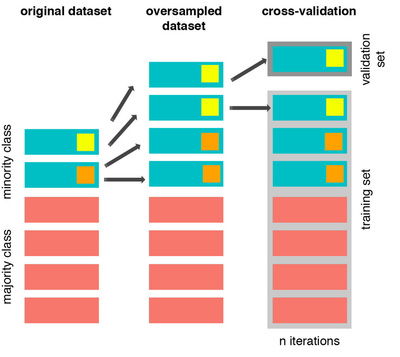
As mentioned previously, if we get the minority class (“Fraud) in our case, and create the synthetic points before cross validating we have a certain influence on the “validation set” of the cross validation process. Remember how cross validation works, let’s assume we are splitting the data into 5 batches, 4/5 of the dataset will be the training set while 1/5 will be the validation set. The test set should not be touched! For that reason, we have to do the creation of synthetic datapoints “during” cross-validation and not before, just like below:
The Right Way:
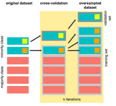
As you see above, SMOTE occurs “during” cross validation and not “prior” to the cross validation process. Synthetic data are created only for the training set without affecting the validation set.
References:
- DEALING WITH IMBALANCED DATA: UNDERSAMPLING, OVERSAMPLING AND PROPER CROSS-VALIDATION
- SMOTE explained for noobs
- Machine Learning - Over-& Undersampling - Python/ Scikit/ Scikit-Imblearn
from imblearn.over_sampling import SMOTE
from sklearn.model_selection import train_test_split, RandomizedSearchCV


print('Length of X (train): {} | Length of y (train): {}'.format(len(original_Xtrain), len(original_ytrain)))
print('Length of X (test): {} | Length of y (test): {}'.format(len(original_Xtest), len(original_ytest)))

# List to append the score and then find the average
accuracy_lst = []
precision_lst = []
recall_lst = []
f1_lst = []
auc_lst = []

# Classifier with optimal parameters
# log_reg_sm = grid_log_reg.best_estimator_
log_reg_sm = LogisticRegression()


rand_log_reg = RandomizedSearchCV(LogisticRegression(), log_reg_params, n_iter=4)


# Implementing SMOTE Technique
# Cross Validating the right way
# Parameters
log_reg_params = {"penalty": ['l1', 'l2'], 'C': [0.001, 0.01, 0.1, 1, 10, 100, 1000]}
for train, test in sss.split(original_Xtrain, original_ytrain):
    pipeline = imbalanced_make_pipeline(SMOTE(sampling_strategy='minority'), rand_log_reg) # SMOTE happens during Cross Validation not before..
    model = pipeline.fit(original_Xtrain[train], original_ytrain[train])
    best_est = rand_log_reg.best_estimator_
    prediction = best_est.predict(original_Xtrain[test])

    accuracy_lst.append(pipeline.score(original_Xtrain[test], original_ytrain[test]))
    precision_lst.append(precision_score(original_ytrain[test], prediction))
    recall_lst.append(recall_score(original_ytrain[test], prediction))
    f1_lst.append(f1_score(original_ytrain[test], prediction))
    auc_lst.append(roc_auc_score(original_ytrain[test], prediction))

print('---' * 45)
print('')
print("accuracy: {}".format(np.mean(accuracy_lst)))
print("precision: {}".format(np.mean(precision_lst)))
print("recall: {}".format(np.mean(recall_lst)))
print("f1: {}".format(np.mean(f1_lst)))
print('---' * 45)
Length of X (train): 227846 | Length of y (train): 227846
Length of X (test): 56961 | Length of y (test): 56961
---------------------------------------------------------------------------------------------------------------------------------------

accuracy: 0.9429314114380596
precision: 0.06252759950989174
recall: 0.9137617656604998
f1: 0.11520272714033197
---------------------------------------------------------------------------------------------------------------------------------------
labels = ['No Fraud', 'Fraud']
smote_prediction = best_est.predict(original_Xtest)
print(classification_report(original_ytest, smote_prediction, target_names=labels))
              precision    recall  f1-score   support

    No Fraud       1.00      0.99      0.99     56863
       Fraud       0.11      0.86      0.20        98

    accuracy                           0.99     56961
   macro avg       0.56      0.92      0.60     56961
weighted avg       1.00      0.99      0.99     56961
y_score = best_est.decision_function(original_Xtest)
average_precision = average_precision_score(original_ytest, y_score)

print('Average precision-recall score: {0:0.2f}'.format(
      average_precision))
Average precision-recall score: 0.75
fig = plt.figure(figsize=(12,6))

precision, recall, _ = precision_recall_curve(original_ytest, y_score)

plt.step(recall, precision, color='r', alpha=0.2,
         where='post')
plt.fill_between(recall, precision, step='post', alpha=0.2,
                 color='#F59B00')

plt.xlabel('Recall')
plt.ylabel('Precision')
plt.ylim([0.0, 1.05])
plt.xlim([0.0, 1.0])
plt.title('OverSampling Precision-Recall curve: \n Average Precision-Recall Score ={0:0.2f}'.format(
          average_precision), fontsize=16)
Text(0.5, 1.0, 'OverSampling Precision-Recall curve: \n Average Precision-Recall Score =0.75')

# SMOTE Technique (OverSampling) After splitting and Cross Validating
#sm = SMOTE(ratio='minority', random_state=42)
sm = SMOTE(sampling_strategy='auto', random_state=42)

# Xsm_train, ysm_train = sm.fit_sample(X_train, y_train)


# This will be the data were we are going to
Xsm_train, ysm_train = sm.fit_resample(original_Xtrain, original_ytrain)
# We Improve the score by 2% points approximately
# Implement GridSearchCV and the other models.

# Logistic Regression
t0 = time.time()
log_reg_sm = grid_log_reg.best_estimator_
log_reg_sm.fit(Xsm_train, ysm_train)
t1 = time.time()
print("Fitting oversample data took :{} sec".format(t1 - t0))
Fitting oversample data took :7.0485217571258545 sec
Test Data with Logistic Regression:
Confusion Matrix:
Positive/Negative: Type of Class (label) [“No”, “Yes”]
True/False: Correctly or Incorrectly classified by the model.
True Negatives (Top-Left Square): This is the number of correctly classifications of the “No” (No Fraud Detected) class.
False Negatives (Top-Right Square): This is the number of incorrectly classifications of the “No”(No Fraud Detected) class.
False Positives (Bottom-Left Square): This is the number of incorrectly classifications of the “Yes” (Fraud Detected) class
True Positives (Bottom-Right Square): This is the number of correctly classifications of the “Yes” (Fraud Detected) class.
Summary:
- Random UnderSampling: We will evaluate the final performance of the classification models in the random undersampling subset. Keep in mind that this is not the data from the original dataframe.
- Classification Models: The models that performed the best were logistic regression and support vector classifier (SVM)
from sklearn.metrics import confusion_matrix

# Logistic Regression fitted using SMOTE technique
y_pred_log_reg = log_reg_sm.predict(X_test)

# Other models fitted with UnderSampling
y_pred_knear = knears_neighbors.predict(X_test)
y_pred_svc = svc.predict(X_test)
y_pred_tree = tree_clf.predict(X_test)


log_reg_cf = confusion_matrix(y_test, y_pred_log_reg)
kneighbors_cf = confusion_matrix(y_test, y_pred_knear)
svc_cf = confusion_matrix(y_test, y_pred_svc)
tree_cf = confusion_matrix(y_test, y_pred_tree)

fig, ax = plt.subplots(2, 2,figsize=(22,12))


sns.heatmap(log_reg_cf, ax=ax[0][0], annot=True, cmap=plt.cm.copper)
ax[0, 0].set_title("Logistic Regression \n Confusion Matrix", fontsize=14)
ax[0, 0].set_xticklabels(['', ''], fontsize=14, rotation=90)
ax[0, 0].set_yticklabels(['', ''], fontsize=14, rotation=360)

sns.heatmap(kneighbors_cf, ax=ax[0][1], annot=True, cmap=plt.cm.copper)
ax[0][1].set_title("KNearsNeighbors \n Confusion Matrix", fontsize=14)
ax[0][1].set_xticklabels(['', ''], fontsize=14, rotation=90)
ax[0][1].set_yticklabels(['', ''], fontsize=14, rotation=360)

sns.heatmap(svc_cf, ax=ax[1][0], annot=True, cmap=plt.cm.copper)
ax[1][0].set_title("Suppor Vector Classifier \n Confusion Matrix", fontsize=14)
ax[1][0].set_xticklabels(['', ''], fontsize=14, rotation=90)
ax[1][0].set_yticklabels(['', ''], fontsize=14, rotation=360)

sns.heatmap(tree_cf, ax=ax[1][1], annot=True, cmap=plt.cm.copper)
ax[1][1].set_title("DecisionTree Classifier \n Confusion Matrix", fontsize=14)
ax[1][1].set_xticklabels(['', ''], fontsize=14, rotation=90)
ax[1][1].set_yticklabels(['', ''], fontsize=14, rotation=360)


plt.show()

from sklearn.metrics import classification_report


print('Logistic Regression:')
print(classification_report(y_test, y_pred_log_reg))

print('KNears Neighbors:')
print(classification_report(y_test, y_pred_knear))

print('Support Vector Classifier:')
print(classification_report(y_test, y_pred_svc))

print('Support Vector Classifier:')
print(classification_report(y_test, y_pred_tree))
Logistic Regression:
              precision    recall  f1-score   support

           0       0.90      0.98      0.94        96
           1       0.98      0.89      0.93        93

    accuracy                           0.94       189
   macro avg       0.94      0.94      0.94       189
weighted avg       0.94      0.94      0.94       189

KNears Neighbors:
              precision    recall  f1-score   support

           0       0.90      0.98      0.94        96
           1       0.98      0.89      0.93        93

    accuracy                           0.94       189
   macro avg       0.94      0.94      0.94       189
weighted avg       0.94      0.94      0.94       189

Support Vector Classifier:
              precision    recall  f1-score   support

           0       0.90      1.00      0.95        96
           1       1.00      0.88      0.94        93

    accuracy                           0.94       189
   macro avg       0.95      0.94      0.94       189
weighted avg       0.95      0.94      0.94       189

Support Vector Classifier:
              precision    recall  f1-score   support

           0       0.86      0.98      0.92        96
           1       0.97      0.84      0.90        93

    accuracy                           0.91       189
   macro avg       0.92      0.91      0.91       189
weighted avg       0.92      0.91      0.91       189
# Final Score in the test set of logistic regression
from sklearn.metrics import accuracy_score

# Logistic Regression with Under-Sampling
y_pred = log_reg.predict(X_test)
undersample_score = accuracy_score(y_test, y_pred)


# Logistic Regression with SMOTE Technique (Better accuracy with SMOTE t)
y_pred_sm = best_est.predict(original_Xtest)
oversample_score = accuracy_score(original_ytest, y_pred_sm)


d = {'Technique': ['Random UnderSampling', 'Oversampling (SMOTE)'], 'Score': [undersample_score, oversample_score]}
final_df = pd.DataFrame(data=d)

# Move column
score = final_df['Score']
final_df.drop('Score', axis=1, inplace=True)
final_df.insert(1, 'Score', score)

# Note how high is accuracy score it can be misleading!
final_df
출력 보기(클릭)
| Technique | Score | |
|---|---|---|
| 0 | Random UnderSampling | 0.936508 |
| 1 | Oversampling (SMOTE) | 0.987992 |
Neural Networks Testing Random UnderSampling Data vs OverSampling (SMOTE):
In this section we will implement a simple Neural Network (with one hidden layer) in order to see which of the two logistic regressions models we implemented in the (undersample or oversample(SMOTE)) has a better accuracy for detecting fraud and non-fraud transactions.
Our Main Goal:
Our main goal is to explore how our simple neural network behaves in both the random undersample and oversample dataframes and see whether they can predict accuractely both non-fraud and fraud cases. Why not only focus on fraud? Imagine you were a cardholder and after you purchased an item your card gets blocked because the bank’s algorithm thought your purchase was a fraud. That’s why we shouldn’t emphasize only in detecting fraud cases but we should also emphasize correctly categorizing non-fraud transactions.
The Confusion Matrix:
Here is again, how the confusion matrix works:
- Upper Left Square: The amount of correctly classified by our model of no fraud transactions.
- Upper Right Square: The amount of incorrectly classified transactions as fraud cases, but the actual label is no fraud .
- Lower Left Square: The amount of incorrectly classified transactions as no fraud cases, but the actual label is fraud .
- Lower Right Square: The amount of correctly classified by our model of fraud transactions.
Summary (Keras || Random UnderSampling):
- Dataset: In this final phase of testing we will fit this model in both the random undersampled subset and oversampled dataset (SMOTE) in order to predict the final result using the original dataframe testing data.
- Neural Network Structure: As stated previously, this will be a simple model composed of one input layer (where the number of nodes equals the number of features) plus bias node, one hidden layer with 32 nodes and one output node composed of two possible results 0 or 1 (No fraud or fraud).
- Other characteristics: The learning rate will be 0.001, the optimizer we will use is the AdamOptimizer, the activation function that is used in this scenario is "Relu" and for the final outputs we will use sparse categorical cross entropy, which gives the probability whether an instance case is no fraud or fraud (The prediction will pick the highest probability between the two.)
import keras
from keras import backend as K
from keras.models import Sequential
from keras.layers import Activation
from keras.layers.core import Dense
from keras.optimizers import Adam
from keras.metrics import categorical_crossentropy

n_inputs = X_train.shape[1]

undersample_model = Sequential([
    Dense(n_inputs, input_shape=(n_inputs, ), activation='relu'),
    Dense(32, activation='relu'),
    Dense(2, activation='softmax')
])
undersample_model.summary()
Model: "sequential"
_________________________________________________________________
 Layer (type)                Output Shape              Param #
=================================================================
 dense (Dense)               (None, 30)                930

 dense_1 (Dense)             (None, 32)                992

 dense_2 (Dense)             (None, 2)                 66

=================================================================
Total params: 1,988
Trainable params: 1,988
Non-trainable params: 0
_________________________________________________________________
undersample_model.compile(Adam(lr=0.001), loss='sparse_categorical_crossentropy', metrics=['accuracy'])
undersample_model.fit(X_train, y_train, validation_split=0.2, batch_size=25, epochs=20, shuffle=True, verbose=2)
Epoch 1/20
25/25 - 2s - loss: 0.6606 - accuracy: 0.5662 - val_loss: 0.4294 - val_accuracy: 0.7020 - 2s/epoch - 83ms/step
Epoch 2/20
25/25 - 0s - loss: 0.3961 - accuracy: 0.7980 - val_loss: 0.2999 - val_accuracy: 0.9205 - 103ms/epoch - 4ms/step
Epoch 3/20
25/25 - 0s - loss: 0.2949 - accuracy: 0.9156 - val_loss: 0.2266 - val_accuracy: 0.9603 - 97ms/epoch - 4ms/step
Epoch 4/20
25/25 - 0s - loss: 0.2320 - accuracy: 0.9288 - val_loss: 0.1779 - val_accuracy: 0.9603 - 98ms/epoch - 4ms/step
Epoch 5/20
25/25 - 0s - loss: 0.1913 - accuracy: 0.9371 - val_loss: 0.1501 - val_accuracy: 0.9603 - 101ms/epoch - 4ms/step
Epoch 6/20
25/25 - 0s - loss: 0.1646 - accuracy: 0.9437 - val_loss: 0.1298 - val_accuracy: 0.9603 - 98ms/epoch - 4ms/step
Epoch 7/20
25/25 - 0s - loss: 0.1464 - accuracy: 0.9487 - val_loss: 0.1177 - val_accuracy: 0.9536 - 97ms/epoch - 4ms/step
Epoch 8/20
25/25 - 0s - loss: 0.1337 - accuracy: 0.9570 - val_loss: 0.1110 - val_accuracy: 0.9536 - 107ms/epoch - 4ms/step
Epoch 9/20
25/25 - 0s - loss: 0.1243 - accuracy: 0.9586 - val_loss: 0.1033 - val_accuracy: 0.9536 - 84ms/epoch - 3ms/step
Epoch 10/20
25/25 - 0s - loss: 0.1174 - accuracy: 0.9603 - val_loss: 0.1009 - val_accuracy: 0.9603 - 88ms/epoch - 4ms/step
Epoch 11/20
25/25 - 0s - loss: 0.1096 - accuracy: 0.9603 - val_loss: 0.0979 - val_accuracy: 0.9603 - 86ms/epoch - 3ms/step
Epoch 12/20
25/25 - 0s - loss: 0.1034 - accuracy: 0.9636 - val_loss: 0.0963 - val_accuracy: 0.9669 - 91ms/epoch - 4ms/step
Epoch 13/20
25/25 - 0s - loss: 0.0984 - accuracy: 0.9652 - val_loss: 0.0933 - val_accuracy: 0.9669 - 84ms/epoch - 3ms/step
Epoch 14/20
25/25 - 0s - loss: 0.0929 - accuracy: 0.9685 - val_loss: 0.0924 - val_accuracy: 0.9603 - 86ms/epoch - 3ms/step
Epoch 15/20
25/25 - 0s - loss: 0.0887 - accuracy: 0.9685 - val_loss: 0.0911 - val_accuracy: 0.9603 - 87ms/epoch - 3ms/step
Epoch 16/20
25/25 - 0s - loss: 0.0849 - accuracy: 0.9719 - val_loss: 0.0892 - val_accuracy: 0.9603 - 84ms/epoch - 3ms/step
Epoch 17/20
25/25 - 0s - loss: 0.0806 - accuracy: 0.9719 - val_loss: 0.0895 - val_accuracy: 0.9669 - 91ms/epoch - 4ms/step
Epoch 18/20
25/25 - 0s - loss: 0.0780 - accuracy: 0.9752 - val_loss: 0.0886 - val_accuracy: 0.9603 - 83ms/epoch - 3ms/step
Epoch 19/20
25/25 - 0s - loss: 0.0740 - accuracy: 0.9768 - val_loss: 0.0917 - val_accuracy: 0.9669 - 87ms/epoch - 3ms/step
Epoch 20/20
25/25 - 0s - loss: 0.0713 - accuracy: 0.9735 - val_loss: 0.0892 - val_accuracy: 0.9669 - 84ms/epoch - 3ms/step


<keras.callbacks.History at 0x157090d5988>
undersample_predictions = undersample_model.predict(original_Xtest, batch_size=200, verbose=0)
undersample_fraud_proba = undersample_model.predict(original_Xtest, batch_size=200, verbose=0) # 예측 확률값 계산
undersample_fraud_predictions = np.argmax(undersample_fraud_proba, axis=1) # 예측 클래스 결정
import itertools

# Create a confusion matrix
def plot_confusion_matrix(cm, classes,
                          normalize=False,
                          title='Confusion matrix',
                          cmap=plt.cm.Blues):
    """
    This function prints and plots the confusion matrix.
    Normalization can be applied by setting `normalize=True`.
    """
    if normalize:
        cm = cm.astype('float') / cm.sum(axis=1)[:, np.newaxis]
        print("Normalized confusion matrix")
    else:
        print('Confusion matrix, without normalization')

    print(cm)

    plt.imshow(cm, interpolation='nearest', cmap=cmap)
    plt.title(title, fontsize=14)
    plt.colorbar()
    tick_marks = np.arange(len(classes))
    plt.xticks(tick_marks, classes, rotation=45)
    plt.yticks(tick_marks, classes)

    fmt = '.2f' if normalize else 'd'
    thresh = cm.max() / 2.
    for i, j in itertools.product(range(cm.shape[0]), range(cm.shape[1])):
        plt.text(j, i, format(cm[i, j], fmt),
                 horizontalalignment="center",
                 color="white" if cm[i, j] > thresh else "black")

    plt.tight_layout()
    plt.ylabel('True label')
    plt.xlabel('Predicted label')
undersample_cm = confusion_matrix(original_ytest, undersample_fraud_predictions)
actual_cm = confusion_matrix(original_ytest, original_ytest)
labels = ['No Fraud', 'Fraud']

fig = plt.figure(figsize=(16,8))

fig.add_subplot(221)
plot_confusion_matrix(undersample_cm, labels, title="Random UnderSample \n Confusion Matrix", cmap=plt.cm.Reds)

fig.add_subplot(222)
plot_confusion_matrix(actual_cm, labels, title="Confusion Matrix \n (with 100% accuracy)", cmap=plt.cm.Greens)
Confusion matrix, without normalization
[[54616  2247]
 [    5    93]]
Confusion matrix, without normalization
[[56863     0]
 [    0    98]]

Keras || OverSampling (SMOTE):
n_inputs = Xsm_train.shape[1]

oversample_model = Sequential([
    Dense(n_inputs, input_shape=(n_inputs, ), activation='relu'),
    Dense(32, activation='relu'),
    Dense(2, activation='softmax')
])
oversample_model.compile(Adam(lr=0.001), loss='sparse_categorical_crossentropy', metrics=['accuracy'])
oversample_model.fit(Xsm_train, ysm_train, validation_split=0.2, batch_size=300, epochs=20, shuffle=True, verbose=2)
Epoch 1/20
1214/1214 - 4s - loss: 0.0729 - accuracy: 0.9737 - val_loss: 0.0314 - val_accuracy: 0.9903 - 4s/epoch - 4ms/step
Epoch 2/20
1214/1214 - 3s - loss: 0.0144 - accuracy: 0.9966 - val_loss: 0.0061 - val_accuracy: 0.9998 - 3s/epoch - 3ms/step
Epoch 3/20
1214/1214 - 3s - loss: 0.0079 - accuracy: 0.9982 - val_loss: 0.0054 - val_accuracy: 0.9998 - 3s/epoch - 3ms/step
Epoch 4/20
1214/1214 - 3s - loss: 0.0053 - accuracy: 0.9989 - val_loss: 0.0022 - val_accuracy: 1.0000 - 3s/epoch - 3ms/step
Epoch 5/20
1214/1214 - 3s - loss: 0.0042 - accuracy: 0.9992 - val_loss: 0.0044 - val_accuracy: 0.9999 - 3s/epoch - 3ms/step
Epoch 6/20
1214/1214 - 3s - loss: 0.0035 - accuracy: 0.9993 - val_loss: 0.0030 - val_accuracy: 1.0000 - 3s/epoch - 3ms/step
Epoch 7/20
1214/1214 - 3s - loss: 0.0030 - accuracy: 0.9994 - val_loss: 8.4192e-04 - val_accuracy: 1.0000 - 3s/epoch - 3ms/step
Epoch 8/20
1214/1214 - 3s - loss: 0.0027 - accuracy: 0.9995 - val_loss: 0.0025 - val_accuracy: 0.9998 - 3s/epoch - 3ms/step
Epoch 9/20
1214/1214 - 3s - loss: 0.0023 - accuracy: 0.9995 - val_loss: 0.0056 - val_accuracy: 0.9981 - 3s/epoch - 3ms/step
Epoch 10/20
1214/1214 - 3s - loss: 0.0022 - accuracy: 0.9995 - val_loss: 0.0011 - val_accuracy: 1.0000 - 3s/epoch - 3ms/step
Epoch 11/20
1214/1214 - 3s - loss: 0.0018 - accuracy: 0.9996 - val_loss: 0.0052 - val_accuracy: 0.9986 - 3s/epoch - 3ms/step
Epoch 12/20
1214/1214 - 3s - loss: 0.0020 - accuracy: 0.9996 - val_loss: 5.1910e-04 - val_accuracy: 1.0000 - 3s/epoch - 3ms/step
Epoch 13/20
1214/1214 - 3s - loss: 0.0017 - accuracy: 0.9997 - val_loss: 5.2539e-04 - val_accuracy: 1.0000 - 3s/epoch - 3ms/step
Epoch 14/20
1214/1214 - 3s - loss: 0.0015 - accuracy: 0.9997 - val_loss: 2.3989e-04 - val_accuracy: 1.0000 - 3s/epoch - 3ms/step
Epoch 15/20
1214/1214 - 3s - loss: 0.0014 - accuracy: 0.9997 - val_loss: 2.3781e-04 - val_accuracy: 1.0000 - 3s/epoch - 3ms/step
Epoch 16/20
1214/1214 - 4s - loss: 0.0013 - accuracy: 0.9997 - val_loss: 2.5659e-04 - val_accuracy: 1.0000 - 4s/epoch - 4ms/step
Epoch 17/20
1214/1214 - 5s - loss: 0.0013 - accuracy: 0.9997 - val_loss: 8.1755e-04 - val_accuracy: 0.9999 - 5s/epoch - 4ms/step
Epoch 18/20
1214/1214 - 4s - loss: 0.0014 - accuracy: 0.9997 - val_loss: 0.0019 - val_accuracy: 0.9999 - 4s/epoch - 3ms/step
Epoch 19/20
1214/1214 - 3s - loss: 9.0269e-04 - accuracy: 0.9998 - val_loss: 2.1974e-04 - val_accuracy: 1.0000 - 3s/epoch - 3ms/step
Epoch 20/20
1214/1214 - 4s - loss: 0.0011 - accuracy: 0.9997 - val_loss: 4.4519e-04 - val_accuracy: 1.0000 - 4s/epoch - 3ms/step


<keras.callbacks.History at 0x15709109208>
oversample_predictions = oversample_model.predict(original_Xtest, batch_size=200, verbose=0)
oversample_fraud_proba = oversample_model.predict(original_Xtest, batch_size=200, verbose=0) # 예측 확률값 계산
oversample_fraud_predictions = np.argmax(oversample_fraud_proba, axis=1) # 예측 클래스 결정
oversample_smote = confusion_matrix(original_ytest, oversample_fraud_predictions)
actual_cm = confusion_matrix(original_ytest, original_ytest)
labels = ['No Fraud', 'Fraud']

fig = plt.figure(figsize=(16,8))

fig.add_subplot(221)
plot_confusion_matrix(oversample_smote, labels, title="OverSample (SMOTE) \n Confusion Matrix", cmap=plt.cm.Oranges)

fig.add_subplot(222)
plot_confusion_matrix(actual_cm, labels, title="Confusion Matrix \n (with 100% accuracy)", cmap=plt.cm.Greens)
Confusion matrix, without normalization
[[56844    19]
 [   27    71]]
Confusion matrix, without normalization
[[56863     0]
 [    0    98]]

Conclusion:
Implementing SMOTE on our imbalanced dataset helped us with the imbalance of our labels (more no fraud than fraud transactions). Nevertheless, I still have to state that sometimes the neural network on the oversampled dataset predicts less correct fraud transactions than our model using the undersample dataset. However, remember that the removal of outliers was implemented only on the random undersample dataset and not on the oversampled one. Also, in our undersample data our model is unable to detect for a large number of cases non fraud transactions correctly and instead, misclassifies those non fraud transactions as fraud cases. Imagine that people that were making regular purchases got their card blocked due to the reason that our model classified that transaction as a fraud transaction, this will be a huge disadvantage for the financial institution. The number of customer complaints and customer disatisfaction will increase. The next step of this analysis will be to do an outlier removal on our oversample dataset and see if our accuracy in the test set improves.
Note: One last thing, predictions and accuracies may be subjected to change since I implemented data shuffling on both types of dataframes. The main thing is to see if our models are able to correctly classify no fraud and fraud transactions. I will bring more updates, stay tuned!